1. 引言：AI编程新时代

人工智能(AI)正在重塑我们的世界，从智能助手到自动驾驶汽车，从医疗诊断到金融预测。AI编程已成为21世纪最具价值的技能之一。本指南将带你从零开始，逐步掌握AI编程的核心概念、工具和实践技巧，无论你是编程新手还是有经验的开发者，都能从中受益。

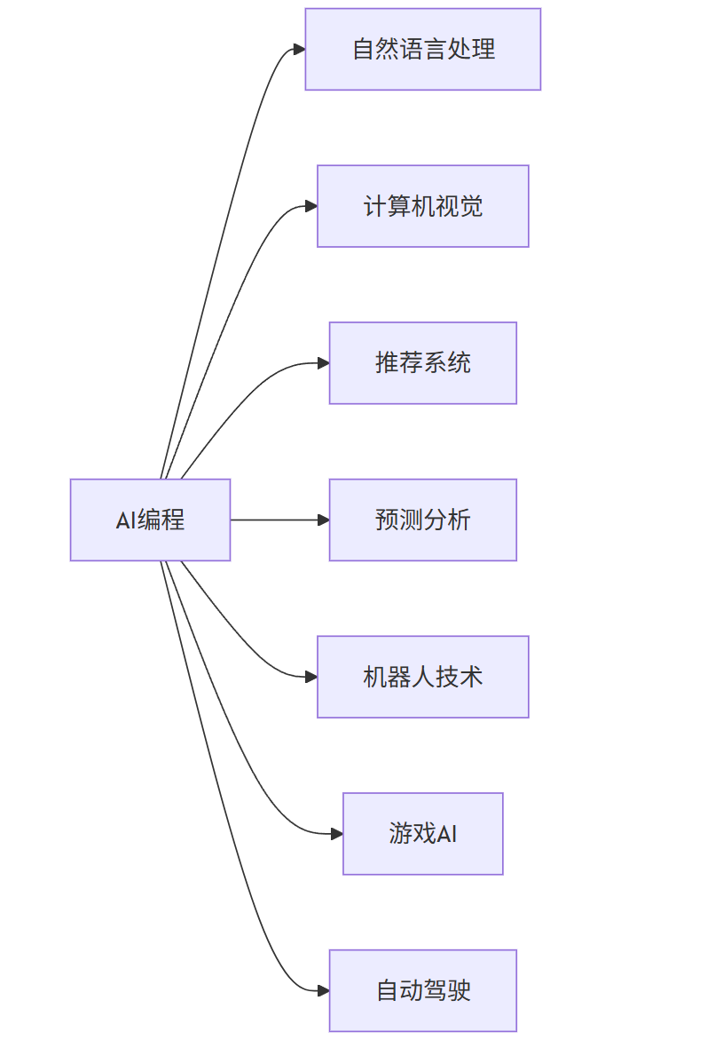
1.1 AI编程的应用领域

graph LR
    A[AI编程] --> B[自然语言处理]
    A --> C[计算机视觉]
    A --> D[推荐系统]
    A --> E[预测分析]
    A --> F[机器人技术]
    A --> G[游戏AI]
    A --> H[自动驾驶]

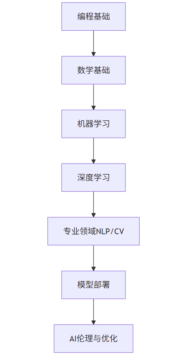
1.2 学习路径概览

flowchart TD
    A[编程基础] --> B[数学基础]
    B --> C[机器学习]
    C --> D[深度学习]
    D --> E[专业领域NLP/CV]
    E --> F[模型部署]
    F --> G[AI伦理与优化]

2. 编程基础：Python与AI生态

Python是AI编程的首选语言，拥有丰富的库和框架支持。让我们从Python基础开始。

2.1 Python基础语法

# 变量和数据类型
name = "AI Learner"
age = 25
height = 1.75
is_student = True

# 列表和字典
languages = ["Python", "R", "Java"]
profile = {"name": "AI Learner", "age": 25, "skills": ["Python", "Machine Learning"]}

# 控制流
if age >= 18:
    print("Adult")
else:
    print("Minor")

# 循环
for lang in languages:
    print(f"I'm learning {lang}")

# 函数
def greet(name):
    return f"Hello, {name}! Welcome to AI programming."

print(greet("Alex"))

2.2 关键Python库

库名称	用途	安装命令
NumPy	数值计算	pip install numpy
Pandas	数据处理	pip install pandas
Matplotlib	数据可视化	pip install matplotlib
Scikit-learn	机器学习	pip install scikit-learn
TensorFlow	深度学习	pip install tensorflow
PyTorch	深度学习	pip install torch

2.3 数据处理示例

import numpy as np
import pandas as pd
import matplotlib.pyplot as plt

# 创建NumPy数组
data = np.random.randn(100, 3)  # 100行3列的随机数据

# 转换为Pandas DataFrame
df = pd.DataFrame(data, columns=['Feature1', 'Feature2', 'Feature3'])

# 基本统计
print(df.describe())

# 数据可视化
plt.figure(figsize=(10, 6))
plt.hist(df['Feature1'], bins=20, alpha=0.7, label='Feature1')
plt.hist(df['Feature2'], bins=20, alpha=0.7, label='Feature2')
plt.hist(df['Feature3'], bins=20, alpha=0.7, label='Feature3')
plt.legend()
plt.title('Feature Distribution')
plt.xlabel('Value')
plt.ylabel('Frequency')
plt.show()

3. 数学基础：AI的基石

AI算法建立在数学基础之上，理解这些概念至关重要。

3.1 线性代数

import numpy as np

# 向量
v1 = np.array([1, 2, 3])
v2 = np.array([4, 5, 6])

# 矩阵
A = np.array([[1, 2], [3, 4], [5, 6]])
B = np.array([[7, 8], [9, 10]])

# 矩阵乘法
C = np.dot(A, B)
print("Matrix multiplication:\n", C)

# 特征值和特征向量
eigenvalues, eigenvectors = np.linalg.eig(np.dot(A.T, A))
print("\nEigenvalues:", eigenvalues)
print("Eigenvectors:\n", eigenvectors)

3.2 微积分与优化

# 梯度下降示例
def gradient_descent(f, df, x0, learning_rate=0.1, max_iter=100):
    x = x0
    history = [x]
    for i in range(max_iter):
        grad = df(x)
        x = x - learning_rate * grad
        history.append(x)
    return x, history

# 示例函数 f(x) = x^2 + 5x + 6
def f(x):
    return x**2 + 5*x + 6

def df(x):
    return 2*x + 5

x0 = 10  # 初始点
min_x, history = gradient_descent(f, df, x0)

print(f"Minimum at x = {min_x:.4f}, f(x) = {f(min_x):.4f}")

# 可视化梯度下降过程
import matplotlib.pyplot as plt
x_vals = np.linspace(-10, 10, 100)
y_vals = f(x_vals)

plt.figure(figsize=(10, 6))
plt.plot(x_vals, y_vals, label='f(x) = x² + 5x + 6')
plt.plot(history, [f(x) for x in history], 'ro-', label='Gradient Descent Path')
plt.xlabel('x')
plt.ylabel('f(x)')
plt.title('Gradient Descent Optimization')
plt.legend()
plt.grid(True)
plt.show()

3.3 概率与统计

import numpy as np
import matplotlib.pyplot as plt
from scipy import stats

# 正态分布
mu, sigma = 0, 1  # 均值和标准差
s = np.random.normal(mu, sigma, 1000)

# 直方图和概率密度函数
count, bins, ignored = plt.hist(s, 30, density=True)
plt.plot(bins, 1/(sigma * np.sqrt(2 * np.pi)) * 
         np.exp(- (bins - mu)**2 / (2 * sigma**2)),
         linewidth=2, color='r')
plt.title('Normal Distribution')
plt.show()

# 假设检验
# 生成两组数据
group1 = np.random.normal(5, 1, 100)
group2 = np.random.normal(5.5, 1, 100)

# t检验
t_stat, p_val = stats.ttest_ind(group1, group2)
print(f"T-statistic: {t_stat:.4f}, p-value: {p_val:.4f}")

if p_val < 0.05:
    print("两组数据有显著差异")
else:
    print("两组数据无显著差异")

4. 机器学习基础

机器学习是AI的核心，让我们从监督学习开始。

4.1 监督学习：分类与回归

from sklearn.datasets import load_iris
from sklearn.model_selection import train_test_split
from sklearn.preprocessing import StandardScaler
from sklearn.neighbors import KNeighborsClassifier
from sklearn.metrics import accuracy_score, classification_report

# 加载鸢尾花数据集
iris = load_iris()
X = iris.data
y = iris.target

# 数据分割
X_train, X_test, y_train, y_test = train_test_split(X, y, test_size=0.3, random_state=42)

# 数据标准化
scaler = StandardScaler()
X_train = scaler.fit_transform(X_train)
X_test = scaler.transform(X_test)

# 创建KNN分类器
knn = KNeighborsClassifier(n_neighbors=3)
knn.fit(X_train, y_train)

# 预测
y_pred = knn.predict(X_test)

# 评估
print("Accuracy:", accuracy_score(y_test, y_pred))
print("\nClassification Report:")
print(classification_report(y_test, y_pred, target_names=iris.target_names))

4.2 非监督学习：聚类

from sklearn.datasets import make_blobs
from sklearn.cluster import KMeans
import matplotlib.pyplot as plt

# 生成模拟数据
X, y = make_blobs(n_samples=300, centers=4, cluster_std=0.60, random_state=0)

# K-means聚类
kmeans = KMeans(n_clusters=4, random_state=42)
kmeans.fit(X)
y_kmeans = kmeans.predict(X)

# 可视化
plt.figure(figsize=(10, 6))
plt.scatter(X[:, 0], X[:, 1], c=y_kmeans, s=50, cmap='viridis')
centers = kmeans.cluster_centers_
plt.scatter(centers[:, 0], centers[:, 1], c='red', s=200, alpha=0.75, marker='X')
plt.title('K-means Clustering')
plt.xlabel('Feature 1')
plt.ylabel('Feature 2')
plt.show()

4.3 模型评估与选择

from sklearn.datasets import load_breast_cancer
from sklearn.model_selection import train_test_split, cross_val_score
from sklearn.preprocessing import StandardScaler
from sklearn.linear_model import LogisticRegression
from sklearn.svm import SVC
from sklearn.ensemble import RandomForestClassifier
from sklearn.metrics import roc_curve, auc

# 加载数据
data = load_breast_cancer()
X = data.data
y = data.target

# 数据预处理
X_train, X_test, y_train, y_test = train_test_split(X, y, test_size=0.3, random_state=42)
scaler = StandardScaler()
X_train = scaler.fit_transform(X_train)
X_test = scaler.transform(X_test)

# 模型比较
models = [
    ('Logistic Regression', LogisticRegression(max_iter=10000)),
    ('SVM', SVC(probability=True)),
    ('Random Forest', RandomForestClassifier())
]

plt.figure(figsize=(10, 8))

for name, model in models:
    # 训练模型
    model.fit(X_train, y_train)
    
    # 交叉验证
    scores = cross_val_score(model, X_train, y_train, cv=5)
    print(f"{name} - CV Accuracy: {scores.mean():.4f} (+/- {scores.std()*2:.4f})")
    
    # ROC曲线
    if hasattr(model, 'predict_proba'):
        y_proba = model.predict_proba(X_test)[:, 1]
    else:
        y_proba = model.decision_function(X_test)
    
    fpr, tpr, _ = roc_curve(y_test, y_proba)
    roc_auc = auc(fpr, tpr)
    
    plt.plot(fpr, tpr, label=f'{name} (AUC = {roc_auc:.2f})')

plt.plot([0, 1], [0, 1], 'k--')
plt.xlim([0.0, 1.0])
plt.ylim([0.0, 1.05])
plt.xlabel('False Positive Rate')
plt.ylabel('True Positive Rate')
plt.title('Receiver Operating Characteristic')
plt.legend(loc="lower right")
plt.show()

5. 深度学习入门

深度学习是AI的强大分支，让我们探索神经网络。

5.1 神经网络基础

import tensorflow as tf
from tensorflow.keras.models import Sequential
from tensorflow.keras.layers import Dense
import numpy as np
import matplotlib.pyplot as plt

# 创建模拟数据
X = np.linspace(-1, 1, 1000)
y = 0.5 * X**3 + 0.2 * X**2 - 0.3 * X + np.random.normal(0, 0.1, 1000)

# 构建模型
model = Sequential([
    Dense(32, activation='relu', input_shape=(1,)),
    Dense(32, activation='relu'),
    Dense(1)
])

model.compile(optimizer='adam', loss='mse')

# 训练模型
history = model.fit(X, y, epochs=100, batch_size=32, validation_split=0.2, verbose=0)

# 预测
X_test = np.linspace(-1.5, 1.5, 100)
y_pred = model.predict(X_test)

# 可视化
plt.figure(figsize=(12, 6))
plt.subplot(1, 2, 1)
plt.plot(history.history['loss'], label='Training Loss')
plt.plot(history.history['val_loss'], label='Validation Loss')
plt.title('Model Loss')
plt.xlabel('Epoch')
plt.ylabel('Loss')
plt.legend()

plt.subplot(1, 2, 2)
plt.scatter(X, y, s=5, label='Original Data')
plt.plot(X_test, y_pred, 'r-', label='Neural Network Prediction')
plt.title('Neural Network Regression')
plt.xlabel('X')
plt.ylabel('y')
plt.legend()
plt.tight_layout()
plt.show()

5.2 卷积神经网络(CNN)用于图像分类

import tensorflow as tf
from tensorflow.keras import layers, models
import matplotlib.pyplot as plt

# 加载MNIST数据集
(train_images, train_labels), (test_images, test_labels) = tf.keras.datasets.mnist.load_data()

# 数据预处理
train_images = train_images.reshape((60000, 28, 28, 1)).astype('float32') / 255
test_images = test_images.reshape((10000, 28, 28, 1)).astype('float32') / 255

# 构建CNN模型
model = models.Sequential([
    layers.Conv2D(32, (3, 3), activation='relu', input_shape=(28, 28, 1)),
    layers.MaxPooling2D((2, 2)),
    layers.Conv2D(64, (3, 3), activation='relu'),
    layers.MaxPooling2D((2, 2)),
    layers.Conv2D(64, (3, 3), activation='relu'),
    layers.Flatten(),
    layers.Dense(64, activation='relu'),
    layers.Dense(10, activation='softmax')
])

model.compile(optimizer='adam',
              loss='sparse_categorical_crossentropy',
              metrics=['accuracy'])

# 训练模型
history = model.fit(train_images, train_labels, epochs=5, 
                    validation_data=(test_images, test_labels))

# 评估
test_loss, test_acc = model.evaluate(test_images, test_labels, verbose=0)
print(f"Test accuracy: {test_acc:.4f}")

# 可视化训练过程
plt.figure(figsize=(12, 4))
plt.subplot(1, 2, 1)
plt.plot(history.history['accuracy'], label='Training Accuracy')
plt.plot(history.history['val_accuracy'], label='Validation Accuracy')
plt.title('Accuracy over Epochs')
plt.xlabel('Epoch')
plt.ylabel('Accuracy')
plt.legend()

plt.subplot(1, 2, 2)
plt.plot(history.history['loss'], label='Training Loss')
plt.plot(history.history['val_loss'], label='Validation Loss')
plt.title('Loss over Epochs')
plt.xlabel('Epoch')
plt.ylabel('Loss')
plt.legend()
plt.tight_layout()
plt.show()

5.3 循环神经网络(RNN)用于序列数据

import numpy as np
import tensorflow as tf
from tensorflow.keras.models import Sequential
from tensorflow.keras.layers import SimpleRNN, Dense
import matplotlib.pyplot as plt

# 生成正弦波数据
def generate_sine_wave(num_samples, seq_length):
    x = np.linspace(0, num_samples * np.pi, num_samples * seq_length)
    y = np.sin(x)
    
    # 创建序列
    sequences = []
    next_values = []
    for i in range(num_samples):
        start = i * seq_length
        end = start + seq_length
        sequences.append(y[start:end])
        next_values.append(y[end])
    
    return np.array(sequences), np.array(next_values)

# 参数设置
num_samples = 1000
seq_length = 50
X, y = generate_sine_wave(num_samples, seq_length)

# 数据分割
split = int(0.8 * num_samples)
X_train, X_test = X[:split], X[split:]
y_train, y_test = y[:split], y[split:]

# 重塑数据以适应RNN输入
X_train = X_train.reshape((X_train.shape[0], X_train.shape[1], 1))
X_test = X_test.reshape((X_test.shape[0], X_test.shape[1], 1))

# 构建RNN模型
model = Sequential([
    SimpleRNN(50, activation='relu', input_shape=(seq_length, 1)),
    Dense(1)
])

model.compile(optimizer='adam', loss='mse')

# 训练模型
history = model.fit(X_train, y_train, epochs=20, 
                    validation_data=(X_test, y_test), verbose=0)

# 预测
y_pred = model.predict(X_test)

# 可视化结果
plt.figure(figsize=(12, 6))
plt.plot(y_test, label='True Values')
plt.plot(y_pred, label='Predicted Values')
plt.title('RNN for Sine Wave Prediction')
plt.xlabel('Time Step')
plt.ylabel('Value')
plt.legend()
plt.show()

6. 自然语言处理(NLP)入门

NLP使计算机能够理解和生成人类语言。

6.1 文本预处理

import nltk
from nltk.corpus import stopwords
from nltk.stem import PorterStemmer, WordNetLemmatizer
from nltk.tokenize import word_tokenize
import re

# 下载NLTK资源
nltk.download('punkt')
nltk.download('stopwords')
nltk.download('wordnet')

# 示例文本
text = "Natural Language Processing (NLP) is a subfield of artificial intelligence that focuses on the interaction between computers and human language. It involves developing algorithms and models that enable computers to understand, interpret, and generate human language in a valuable way."

# 转换为小写
text = text.lower()

# 移除标点符号
text = re.sub(r'[^\w\s]', '', text)

# 分词
tokens = word_tokenize(text)

# 移除停用词
stop_words = set(stopwords.words('english'))
filtered_tokens = [word for word in tokens if word not in stop_words]

# 词干提取
stemmer = PorterStemmer()
stemmed_tokens = [stemmer.stem(word) for word in filtered_tokens]

# 词形还原
lemmatizer = WordNetLemmatizer()
lemmatized_tokens = [lemmatizer.lemmatize(word) for word in filtered_tokens]

print("Original Tokens:", tokens[:10])
print("Filtered Tokens:", filtered_tokens[:10])
print("Stemmed Tokens:", stemmed_tokens[:10])
print("Lemmatized Tokens:", lemmatized_tokens[:10])

6.2 情感分析

from textblob import TextBlob
from sklearn.feature_extraction.text import TfidfVectorizer
from sklearn.model_selection import train_test_split
from sklearn.naive_bayes import MultinomialNB
from sklearn.metrics import accuracy_score, classification_report

# 示例数据
texts = [
    "I love this product! It's amazing and works perfectly.",
    "This is the worst experience I've ever had. Terrible service.",
    "The movie was okay, not great but not bad either.",
    "I'm so happy with my purchase. Highly recommended!",
    "The food was disgusting and the staff was rude."
]
labels = [1, 0, 2, 1, 0]  # 1: positive, 0: negative, 2: neutral

# 使用TextBlob进行快速情感分析
for text in texts:
    analysis = TextBlob(text)
    sentiment = "positive" if analysis.sentiment.polarity > 0 else "negative" if analysis.sentiment.polarity < 0 else "neutral"
    print(f"Text: {text}\nSentiment: {sentiment} (Polarity: {analysis.sentiment.polarity:.2f})\n")

# 使用机器学习进行情感分析
# 特征提取
vectorizer = TfidfVectorizer()
X = vectorizer.fit_transform(texts)

# 数据分割
X_train, X_test, y_train, y_test = train_test_split(X, labels, test_size=0.4, random_state=42)

# 训练模型
model = MultinomialNB()
model.fit(X_train, y_train)

# 预测
y_pred = model.predict(X_test)

# 评估
print("\nMachine Learning Model Evaluation:")
print(f"Accuracy: {accuracy_score(y_test, y_pred):.2f}")
print("\nClassification Report:")
print(classification_report(y_test, y_pred, target_names=['negative', 'positive', 'neutral']))

6.3 使用预训练模型：Hugging Face Transformers

from transformers import pipeline

# 情感分析
sentiment_pipeline = pipeline("sentiment-analysis")
result = sentiment_pipeline("I love learning about artificial intelligence!")
print("Sentiment Analysis:", result)

# 文本生成
text_generator = pipeline("text-generation", model="gpt2")
prompt = "In the future, AI will"
generated_text = text_generator(prompt, max_length=30, num_return_sequences=1)
print("\nText Generation:")
print(generated_text[0]['generated_text'])

# 问答
qa_pipeline = pipeline("question-answering")
context = "Artificial intelligence (AI) is intelligence demonstrated by machines, as opposed to natural intelligence displayed by animals including humans. AI research has been defined as the field of study of intelligent agents, which refers to any system that perceives its environment and takes actions that maximize its chance of achieving its goals."
question = "What is AI?"
answer = qa_pipeline(question=question, context=context)
print("\nQuestion Answering:")
print(f"Question: {question}")
print(f"Answer: {answer['answer']}")

7. 计算机视觉入门

计算机视觉使计算机能够理解和解释视觉信息。

7.1 图像处理基础

import cv2
import numpy as np
import matplotlib.pyplot as plt

# 读取图像
image = cv2.imread('example.jpg')  # 替换为实际图像路径
image_rgb = cv2.cvtColor(image, cv2.COLOR_BGR2RGB)  # 转换颜色空间

# 转换为灰度图
gray_image = cv2.cvtColor(image, cv2.COLOR_BGR2GRAY)

# 边缘检测
edges = cv2.Canny(gray_image, 100, 200)

# 显示图像
plt.figure(figsize=(15, 10))
plt.subplot(1, 3, 1)
plt.imshow(image_rgb)
plt.title('Original Image')
plt.axis('off')

plt.subplot(1, 3, 2)
plt.imshow(gray_image, cmap='gray')
plt.title('Grayscale Image')
plt.axis('off')

plt.subplot(1, 3, 3)
plt.imshow(edges, cmap='gray')
plt.title('Edge Detection')
plt.axis('off')

plt.tight_layout()
plt.show()

7.2 目标检测

import cv2
import numpy as np
import matplotlib.pyplot as plt

# 加载预训练的YOLO模型
net = cv2.dnn.readNet("yolov3.weights", "yolov3.cfg")  # 需要下载这些文件
classes = []
with open("coco.names", "r") as f:  # 需要下载这个文件
    classes = [line.strip() for line in f.readlines()]

layer_names = net.getLayerNames()
output_layers = [layer_names[i[0] - 1] for i in net.getUnconnectedOutLayers()]

# 加载图像
image = cv2.imread('example.jpg')  # 替换为实际图像路径
height, width, channels = image.shape

# 预处理图像
blob = cv2.dnn.blobFromImage(image, 0.00392, (416, 416), (0, 0, 0), True, crop=False)
net.setInput(blob)
outs = net.forward(output_layers)

# 处理检测结果
class_ids = []
confidences = []
boxes = []
for out in outs:
    for detection in out:
        scores = detection[5:]
        class_id = np.argmax(scores)
        confidence = scores[class_id]
        if confidence > 0.5:
            # 目标检测
            center_x = int(detection[0] * width)
            center_y = int(detection[1] * height)
            w = int(detection[2] * width)
            h = int(detection[3] * height)
            
            # 矩形坐标
            x = int(center_x - w / 2)
            y = int(center_y - h / 2)
            
            boxes.append([x, y, w, h])
            confidences.append(float(confidence))
            class_ids.append(class_id)

# 非极大值抑制
indexes = cv2.dnn.NMSBoxes(boxes, confidences, 0.5, 0.4)

# 绘制边界框和标签
font = cv2.FONT_HERSHEY_PLAIN
colors = np.random.uniform(0, 255, size=(len(classes), 3))
for i in range(len(boxes)):
    if i in indexes:
        x, y, w, h = boxes[i]
        label = str(classes[class_ids[i]])
        color = colors[class_ids[i]]
        cv2.rectangle(image, (x, y), (x + w, y + h), color, 2)
        cv2.putText(image, label, (x, y + 30), font, 3, color, 3)

# 显示结果
image_rgb = cv2.cvtColor(image, cv2.COLOR_BGR2RGB)
plt.figure(figsize=(12, 8))
plt.imshow(image_rgb)
plt.title('Object Detection with YOLO')
plt.axis('off')
plt.show()

7.3 图像分割

import numpy as np
import matplotlib.pyplot as plt
from skimage import data, segmentation, color
from skimage.future import graph

# 加载示例图像
image = data.coffee()

# 使用SLIC算法进行超像素分割
labels = segmentation.slic(image, compactness=30, n_segments=400)

# 创建区域邻接图
g = graph.rag_mean_color(image, labels)

# 使用归一化切割进行分割
labels2 = graph.cut_normalized(labels, g)

# 显示结果
plt.figure(figsize=(15, 10))
plt.subplot(1, 3, 1)
plt.imshow(image)
plt.title('Original Image')
plt.axis('off')

plt.subplot(1, 3, 2)
plt.imshow(color.label2rgb(labels, image, kind='avg'))
plt.title('Superpixels')
plt.axis('off')

plt.subplot(1, 3, 3)
plt.imshow(color.label2rgb(labels2, image, kind='avg'))
plt.title('Normalized Cut Segmentation')
plt.axis('off')

plt.tight_layout()
plt.show()

8. AI模型部署

训练好的模型需要部署才能实际应用。

8.1 使用Flask部署模型

from flask import Flask, request, jsonify
import numpy as np
import tensorflow as tf
import pickle

app = Flask(__name__)

# 加载模型
model = tf.keras.models.load_model('my_model.h5')  # 替换为实际模型路径

# 加载预处理器
with open('preprocessor.pkl', 'rb') as f:
    preprocessor = pickle.load(f)

@app.route('/predict', methods=['POST'])
def predict():
    # 获取JSON数据
    data = request.json
    
    # 预处理数据
    processed_data = preprocessor.transform(np.array(data['features']).reshape(1, -1))
    
    # 预测
    prediction = model.predict(processed_data)
    
    # 返回结果
    return jsonify({
        'prediction': prediction.tolist(),
        'status': 'success'
    })

if __name__ == '__main__':
    app.run(debug=True)

8.2 使用Docker容器化

# Dockerfile
FROM python:3.8-slim

WORKDIR /app

# 复制依赖文件
COPY requirements.txt .

# 安装依赖
RUN pip install --no-cache-dir -r requirements.txt

# 复制应用代码
COPY . .

# 暴露端口
EXPOSE 5000

# 运行应用
CMD ["python", "app.py"]

8.3 部署到云平台

flowchart TD
    A[训练模型] --> B[保存模型]
    B --> C[创建API服务]
    C --> D[容器化应用]
    D --> E[推送到容器注册表]
    E --> F[部署到云平台]
    F --> G[配置自动扩展]
    G --> H[监控与日志]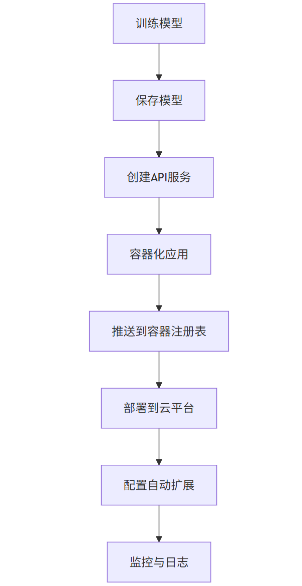

9. Prompt工程入门

与大型语言模型(LLM)交互需要有效的Prompt设计。

9.1 Prompt设计原则

1. 明确具体：清晰表达你的需求
2. 提供上下文：给出足够背景信息
3. 设定角色：指定模型扮演的角色
4. 示例引导：提供输入输出示例
5. 逐步思考：引导模型逐步推理

9.2 Prompt示例

基础Prompt

解释什么是机器学习，用简单的语言。

角色设定Prompt

你是一位经验丰富的数据科学家，向非技术人员解释深度学习的工作原理。

示例引导Prompt

任务：将文本分类为积极、消极或中性情感。
示例：
输入："我非常喜欢这部电影！" 输出：积极
输入："服务太差了，不会再来了。" 输出：消极
输入："食物还可以，价格适中。" 输出：中性
输入："产品质量超出预期，非常满意。" 输出：

逐步思考Prompt

解决以下数学问题，逐步展示你的思考过程：
问题：一个水池有两个进水管和一个出水管。第一个进水管每小时注水10升，第二个进水管每小时注水15升，出水管每小时排水8升。如果水池最初是空的，三个水管同时打开，需要多少小时才能注满50升的水池？

9.3 高级Prompt技巧

import openai

# 设置API密钥
openai.api_key = 'your-api-key'

def generate_response(prompt, temperature=0.7, max_tokens=150):
    response = openai.Completion.create(
        engine="text-davinci-003",
        prompt=prompt,
        temperature=temperature,
        max_tokens=max_tokens,
        top_p=1.0,
        frequency_penalty=0.0,
        presence_penalty=0.0
    )
    return response.choices[0].text.strip()

# 示例1：链式思考Prompt
prompt = """
Q: 罗杰有5个网球。他又买了2罐网球，每罐有3个网球。他现在有多少个网球？
A: 罗杰最初有5个网球。2罐网球，每罐3个，总共是2*3=6个网球。5+6=11。答案是11个网球。

Q: 食堂有23个苹果。他们用20个做了午餐，又买了6个。现在有多少个苹果？
A: 
"""
print(generate_response(prompt))

# 示例2：少样本学习Prompt
prompt = """
将以下文本分类为"体育"、"科技"或"娱乐"：
文本："新的智能手机型号具有革命性的摄像头技术。" 分类：科技
文本："球队在最后时刻赢得了冠军。" 分类：体育
文本："最新电影在上映首周就打破了票房记录。" 分类：娱乐
文本："科学家发现了治疗疾病的新方法。" 分类：
"""
print(generate_response(prompt))

10. AI伦理与负责任开发

AI开发必须考虑伦理和社会影响。

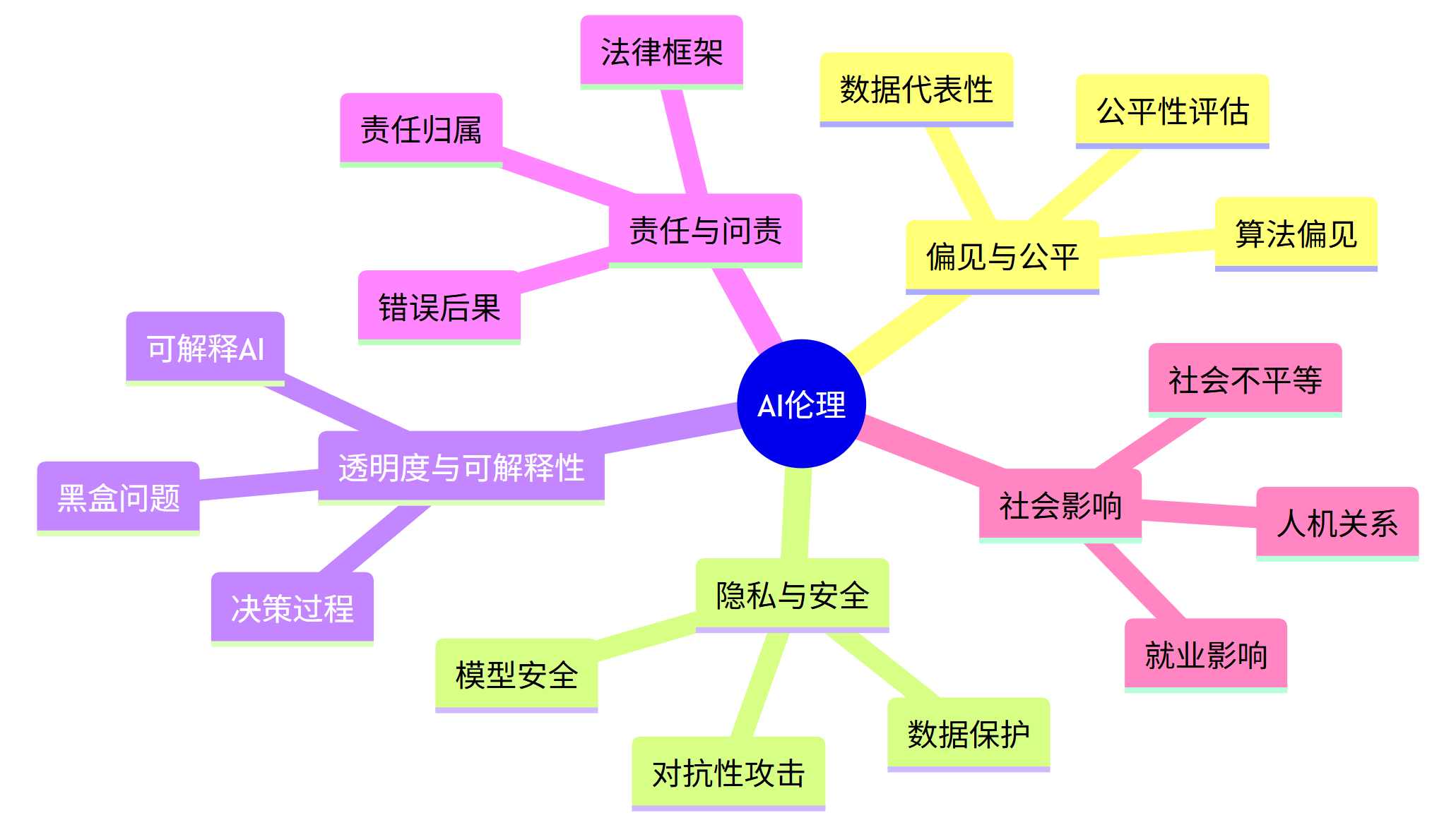
10.1 关键伦理问题

mindmap
  root((AI伦理))
    偏见与公平
      算法偏见
      数据代表性
      公平性评估
    隐私与安全
      数据保护
      模型安全
      对抗性攻击
    透明度与可解释性
      黑盒问题
      可解释AI
      决策过程
    责任与问责
      责任归属
      错误后果
      法律框架
    社会影响
      就业影响
      社会不平等
      人机关系

10.2 负责任AI开发实践

# 示例：检测和减轻数据偏见
import pandas as pd
from sklearn.model_selection import train_test_split
from sklearn.ensemble import RandomForestClassifier
from sklearn.metrics import accuracy_score
from aif360.datasets import BinaryLabelDataset
from aif360.metrics import BinaryLabelDatasetMetric
from aif360.algorithms.preprocessing import Reweighing

# 加载数据
data = pd.read_csv('adult_data.csv')  # 替换为实际数据路径

# 创建二进制标签数据集
privileged_groups = [{'sex': 1}]  # 男性
unprivileged_groups = [{'sex': 0}]  # 女性

binary_label_dataset = BinaryLabelDataset(
    df=data,
    label_names=['income'],
    protected_attribute_names=['sex'],
    favorable_label=1,
    unfavorable_label=0
)

# 计算原始偏见
metric = BinaryLabelDatasetMetric(
    binary_label_dataset,
    unprivileged_groups=unprivileged_groups,
    privileged_groups=privileged_groups
)
print("Original Disparate Impact:", metric.disparate_impact())

# 应用重新加权减轻偏见
RW = Reweighing(
    unprivileged_groups=unprivileged_groups,
    privileged_groups=privileged_groups
)
transformed_dataset = RW.fit_transform(binary_label_dataset)

# 计算减轻偏见后的指标
transformed_metric = BinaryLabelDatasetMetric(
    transformed_dataset,
    unprivileged_groups=unprivileged_groups,
    privileged_groups=privileged_groups
)
print("Transformed Disparate Impact:", transformed_metric.disparate_impact())

# 转换回原始格式并训练模型
transformed_data = transformed_dataset.convert_to_dataframe()[0]
X = transformed_data.drop('income', axis=1)
y = transformed_data['income']

X_train, X_test, y_train, y_test = train_test_split(X, y, test_size=0.3, random_state=42)

# 训练模型
model = RandomForestClassifier(random_state=42)
model.fit(X_train, y_train)

# 评估
y_pred = model.predict(X_test)
print("Model Accuracy:", accuracy_score(y_test, y_pred))

11. 学习资源与社区

持续学习是AI领域的关键。

11.1 推荐学习资源

资源类型	推荐内容
在线课程	Coursera: Andrew Ng的机器学习课程
	fast.ai: 深度学习实战课程
书籍	《Python机器学习》- Sebastian Raschka
	《深度学习》- Ian Goodfellow
框架文档	TensorFlow官方教程
	PyTorch官方教程
研究论文	arXiv.org
	Papers With Code

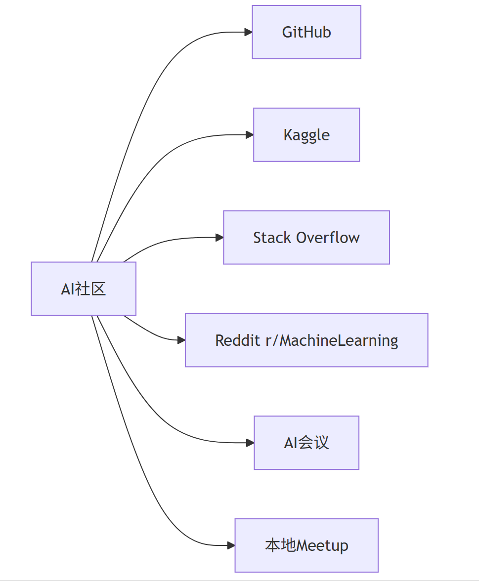
11.2 参与AI社区

graph LR
    A[AI社区] --> B[GitHub]
    A --> C[Kaggle]
    A --> D[Stack Overflow]
    A --> E[Reddit r/MachineLearning]
    A --> F[AI会议]
    A --> G[本地Meetup]

12. 实战项目：构建端到端AI应用

让我们整合所学知识，构建一个完整的AI应用。

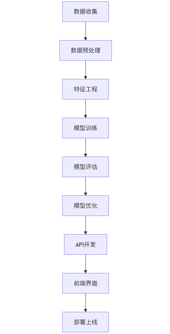
12.1 项目概述：电影评论情感分析系统

flowchart TD
    A[数据收集] --> B[数据预处理]
    B --> C[特征工程]
    C --> D[模型训练]
    D --> E[模型评估]
    E --> F[模型优化]
    F --> G[API开发]
    G --> H[前端界面]
    H --> I[部署上线]

12.2 完整代码实现

# 1. 数据收集与预处理
import pandas as pd
import numpy as np
import re
import nltk
from nltk.corpus import stopwords
from nltk.stem import WordNetLemmatizer
from sklearn.model_selection import train_test_split
from sklearn.feature_extraction.text import TfidfVectorizer
from sklearn.ensemble import RandomForestClassifier
from sklearn.metrics import accuracy_score, classification_report
import pickle
import flask
from flask import Flask, request, jsonify

# 下载NLTK资源
nltk.download('stopwords')
nltk.download('wordnet')

# 加载数据 (假设我们有一个CSV文件包含评论和情感标签)
data = pd.read_csv('movie_reviews.csv')  # 替换为实际数据路径

# 数据预处理
def preprocess_text(text):
    # 转换为小写
    text = text.lower()
    # 移除特殊字符
    text = re.sub(r'[^\w\s]', '', text)
    # 分词
    tokens = text.split()
    # 移除停用词
    stop_words = set(stopwords.words('english'))
    tokens = [word for word in tokens if word not in stop_words]
    # 词形还原
    lemmatizer = WordNetLemmatizer()
    tokens = [lemmatizer.lemmatize(word) for word in tokens]
    return ' '.join(tokens)

data['processed_review'] = data['review'].apply(preprocess_text)

# 特征工程
vectorizer = TfidfVectorizer(max_features=5000)
X = vectorizer.fit_transform(data['processed_review'])
y = data['sentiment']  # 假设情感标签为0或1

# 数据分割
X_train, X_test, y_train, y_test = train_test_split(X, y, test_size=0.2, random_state=42)

# 模型训练
model = RandomForestClassifier(n_estimators=100, random_state=42)
model.fit(X_train, y_train)

# 模型评估
y_pred = model.predict(X_test)
print("Accuracy:", accuracy_score(y_test, y_pred))
print("\nClassification Report:")
print(classification_report(y_test, y_pred))

# 保存模型和向量化器
with open('sentiment_model.pkl', 'wb') as f:
    pickle.dump(model, f)
    
with open('vectorizer.pkl', 'wb') as f:
    pickle.dump(vectorizer, f)

# 2. API开发
app = Flask(__name__)

# 加载模型和向量化器
with open('sentiment_model.pkl', 'rb') as f:
    model = pickle.load(f)
    
with open('vectorizer.pkl', 'rb') as f:
    vectorizer = pickle.load(f)

@app.route('/predict', methods=['POST'])
def predict():
    # 获取评论
    review = request.json['review']
    
    # 预处理
    processed_review = preprocess_text(review)
    
    # 向量化
    vectorized_review = vectorizer.transform([processed_review])
    
    # 预测
    prediction = model.predict(vectorized_review)[0]
    probability = model.predict_proba(vectorized_review)[0].max()
    
    # 返回结果
    sentiment = "positive" if prediction == 1 else "negative"
    return jsonify({
        'review': review,
        'sentiment': sentiment,
        'confidence': float(probability)
    })

if __name__ == '__main__':
    app.run(debug=True)

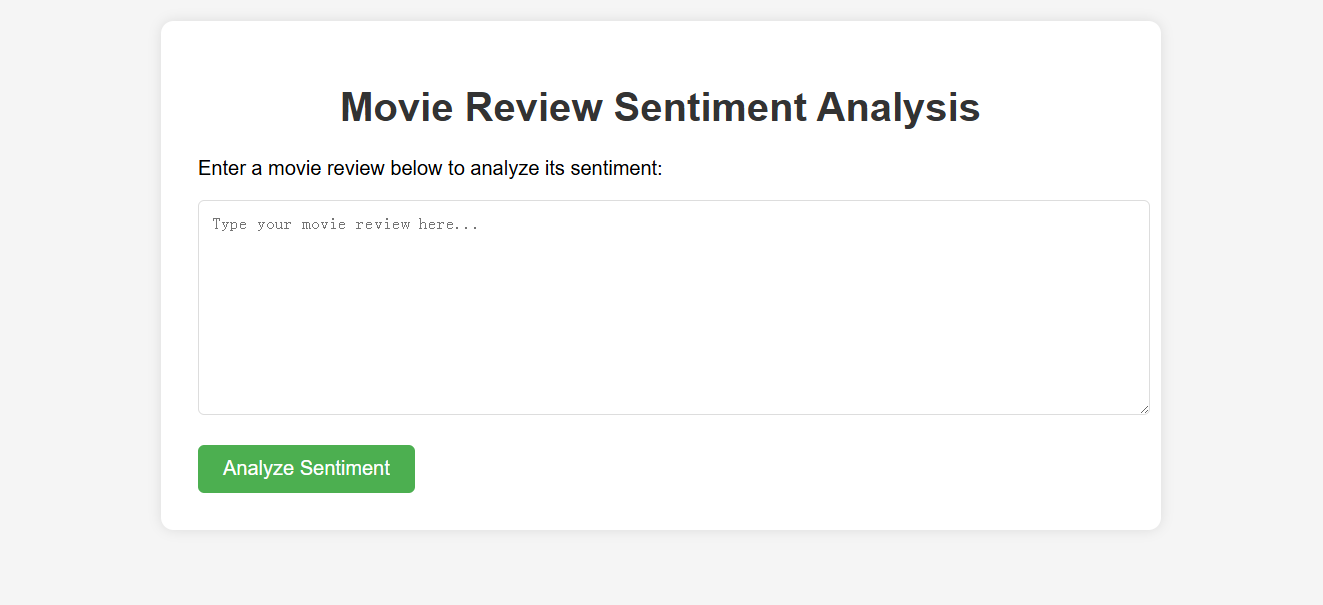
12.3 前端界面示例

<!DOCTYPE html>
<html lang="en">
<head>
    <meta charset="UTF-8">
    <meta name="viewport" content="width=device-width, initial-scale=1.0">
    <title>Movie Review Sentiment Analysis</title>
    <style>
        body {
            font-family: Arial, sans-serif;
            max-width: 800px;
            margin: 0 auto;
            padding: 20px;
            background-color: #f5f5f5;
        }
        .container {
            background-color: white;
            padding: 30px;
            border-radius: 10px;
            box-shadow: 0 0 10px rgba(0,0,0,0.1);
        }
        h1 {
            color: #333;
            text-align: center;
        }
        textarea {
            width: 100%;
            height: 150px;
            padding: 10px;
            margin-bottom: 20px;
            border: 1px solid #ddd;
            border-radius: 5px;
        }
        button {
            background-color: #4CAF50;
            color: white;
            padding: 10px 20px;
            border: none;
            border-radius: 5px;
            cursor: pointer;
            font-size: 16px;
        }
        button:hover {
            background-color: #45a049;
        }
        .result {
            margin-top: 20px;
            padding: 15px;
            border-radius: 5px;
            display: none;
        }
        .positive {
            background-color: #dff0d8;
            color: #3c763d;
        }
        .negative {
            background-color: #f2dede;
            color: #a94442;
        }
    </style>
</head>
<body>
    <div class="container">
        <h1>Movie Review Sentiment Analysis</h1>
        <p>Enter a movie review below to analyze its sentiment:</p>
        <textarea id="review" placeholder="Type your movie review here..."></textarea>
        <button οnclick="analyzeSentiment()">Analyze Sentiment</button>
        <div id="result" class="result"></div>
    </div>

    <script>
        function analyzeSentiment() {
            const review = document.getElementById('review').value;
            const resultDiv = document.getElementById('result');
            
            if (!review.trim()) {
                resultDiv.textContent = "Please enter a review.";
                resultDiv.className = "result";
                resultDiv.style.display = "block";
                return;
            }
            
            fetch('/predict', {
                method: 'POST',
                headers: {
                    'Content-Type': 'application/json',
                },
                body: JSON.stringify({ review: review }),
            })
            .then(response => response.json())
            .then(data => {
                resultDiv.innerHTML = `
                    <strong>Review:</strong> ${data.review}<br>
                    <strong>Sentiment:</strong> ${data.sentiment}<br>
                    <strong>Confidence:</strong> ${(data.confidence * 100).toFixed(2)}%
                `;
                resultDiv.className = `result ${data.sentiment}`;
                resultDiv.style.display = "block";
            })
            .catch(error => {
                console.error('Error:', error);
                resultDiv.textContent = "An error occurred. Please try again.";
                resultDiv.className = "result";
                resultDiv.style.display = "block";
            });
        }
    </script>
</body>
</html>

13. 总结与未来展望

AI编程是一个快速发展的领域，掌握其基础知识和实践技能将为你的职业发展打开无数可能。本指南涵盖了从编程基础到高级AI技术的全面内容，包括：

1. Python编程和AI生态系统
2. 必要的数学基础
3. 机器学习和深度学习核心概念
4. 自然语言处理和计算机视觉应用
5. 模型部署和Prompt工程
6. AI伦理和负责任开发

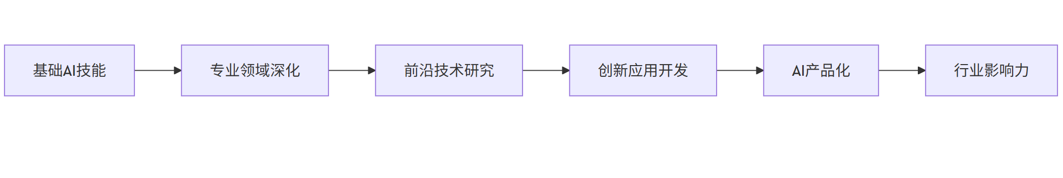
13.1 持续学习路径

flowchart LR
    A[基础AI技能] --> B[专业领域深化]
    B --> C[前沿技术研究]
    C --> D[创新应用开发]
    D --> E[AI产品化]
    E --> F[行业影响力]

13.2 未来趋势

1. 多模态AI：结合文本、图像、音频等多种数据类型的AI系统
2. 自监督学习：减少对标记数据的依赖
3. 小样本学习：用少量数据训练高效模型
4. 可解释AI：提高模型透明度和可信度
5. 边缘AI：在设备端部署轻量级AI模型
6. AI民主化：降低AI开发门槛，使更多人能够参与

13.3 最终建议

1. 动手实践：理论知识需要通过实际项目来巩固
2. 参与社区：加入AI社区，与他人交流学习
3. 保持更新：AI领域发展迅速，持续学习新知识
4. 跨学科学习：结合领域知识（如医疗、金融等）开发专业AI应用
5. 伦理意识：始终考虑AI技术的社会影响和伦理问题

AI编程之旅充满挑战也充满机遇。希望本指南能为你提供坚实的基础，激发你探索AI世界的热情。记住，最好的学习方式是实践——立即开始你的第一个AI项目吧！