第一章机器学习模型与实现

红目香薰

43098人浏览 · 2026-07-13 11:04:32

红目香薰 · 2026-07-13 11:04:32 发布

在这里插入图片描述

环境准备

在开始本章学习之前，请确保已安装以下Python依赖包：

pip install numpy
pip install matplotlib
pip install scikit-learn
pip install pandas

安装说明：

包名	版本要求	用途
numpy	>= 1.21.0	数值计算基础库
matplotlib	>= 3.4.0	数据可视化库
scikit-learn	>= 1.0.0	机器学习算法库
pandas	>= 1.3.0	数据处理库（部分示例使用）

快速安装命令：

pip install numpy matplotlib scikit-learn pandas -i https://pypi.tuna.tsinghua.edu.cn/simple

提示：使用 -i https://pypi.tuna.tsinghua.edu.cn/simple 参数可以通过清华大学镜像源加速安装，适合国内用户。

课程概述

本章将介绍六种经典的机器学习算法，包括线性回归、逻辑回归、神经网络、支持向量机、随机森林和梯度提升决策树（GBDT）。每种算法将从原理、实现和应用三个层面进行讲解，配合Jupyter Notebook代码演示，帮助学员快速掌握机器学习模型的核心概念和实践技能。

总学时：3学时（每节0.5学时）

1.1 线性回归

教学目标

理解线性回归的基本原理和数学模型
掌握使用scikit-learn实现线性回归的方法
理解损失函数和最小二乘法
学会评估线性回归模型的性能

重点难点

重点	难点
线性回归的数学表达式	梯度下降算法原理
最小二乘法求解	过拟合与正则化
模型评估指标	特征缩放的重要性

教学过程（30分钟）

1. 原理讲解（10分钟）

线性回归模型

线性回归是一种用于预测连续值的监督学习算法。其数学表达式为：

$\beta_0 + \beta_1 x_1 + \beta_2 x_2 + \dots + \beta_n x_n + \epsilon$

其中：

$y$ 是预测值
$β0\beta_0$ 是截距项
$β1,β2,…,βn\beta_1, \beta_2, \dots, \beta_n$ 是特征系数
$x1,x2,…,xnx_1, x_2, \dots, x_n$ 是输入特征
$ϵ\epsilon$ 是误差项

损失函数

线性回归使用均方误差（MSE）作为损失函数：

$MSE=1m∑i=1m(yi−y^i)2 \text{MSE} = \frac{1}{m} \sum_{i=1}^{m} (y_i - \hat{y}_i)^2$

求解方法

最小二乘法：通过解析方法直接求解系数
梯度下降法：通过迭代优化寻找最优解

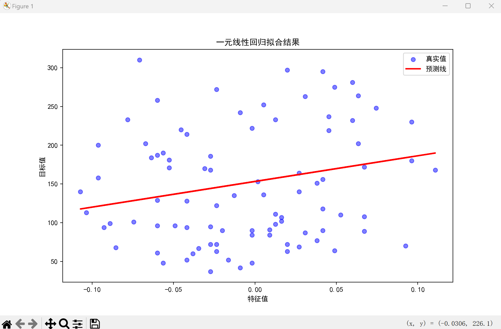
2. 代码演示（15分钟）

import numpy as np
import matplotlib.pyplot as plt
from sklearn.datasets import load_diabetes
from sklearn.linear_model import LinearRegression
from sklearn.model_selection import train_test_split
from sklearn.metrics import mean_squared_error, r2_score

plt.rcParams['font.sans-serif'] = ['SimHei']
plt.rcParams['axes.unicode_minus'] = False

data = load_diabetes()
X = data.data[:, 0].reshape(-1, 1)
y = data.target

X_train, X_test, y_train, y_test = train_test_split(X, y, test_size=0.2, random_state=42)

lr = LinearRegression()
lr.fit(X_train, y_train)

y_pred = lr.predict(X_test)

print("均方误差 MSE =", mean_squared_error(y_test, y_pred))
print("决定系数 R² =", r2_score(y_test, y_pred))

plt.figure(figsize=(10, 6))
plt.scatter(X_test, y_test, color='blue', alpha=0.5, label='真实值')
plt.plot(X_test, y_pred, color='red', linewidth=2, label='预测线')
plt.xlabel('特征值')
plt.ylabel('目标值')
plt.title('一元线性回归拟合结果')
plt.legend()
plt.show()

3. 模型评估（5分钟）

常用评估指标：

均方误差（MSE）：衡量预测值与真实值的平均平方差
R²评分：衡量模型对数据变异的解释程度，取值范围[0,1]

课后思考

线性回归的假设条件有哪些？
如果特征之间存在多重共线性，会对线性回归产生什么影响？
如何处理非线性数据的回归问题？

1.2 逻辑回归

教学目标

理解逻辑回归的基本原理和sigmoid函数
掌握使用scikit-learn实现逻辑回归的方法
理解对数几率和决策边界
学会评估分类模型的性能

重点难点

重点	难点
Sigmoid函数的特性	极大似然估计原理
决策边界的概念	多类别分类的实现
分类评估指标	正则化参数的选择

教学过程（30分钟）

1. 原理讲解（10分钟）

Sigmoid函数

逻辑回归使用sigmoid函数将线性组合转换为概率值：

$\sigma(z) = \frac{1}{1 + e^{-z}}$

其中 $\beta_0 + \beta_1 x_1 + \dots + \beta_n x_n$

预测规则

$y^={1if σ(z)≥0.50if σ(z)<0.5 \hat{y} = \begin{cases} 1 & \text{if } \sigma(z) \geq 0.5 \\ 0 & \text{if } \sigma(z) < 0.5 \end{cases}$

损失函数

逻辑回归使用对数损失（Log Loss）：

$Loss=−1m∑i=1m[yilog⁡(y^i)+(1−yi)log⁡(1−y^i)] \text{Log Loss} = -\frac{1}{m} \sum_{i=1}^{m} [y_i \log(\hat{y}_i) + (1-y_i) \log(1-\hat{y}_i)]$

2. 代码演示（15分钟）

import numpy as np
import matplotlib.pyplot as plt
from sklearn.datasets import load_iris
from sklearn.linear_model import LogisticRegression
from sklearn.model_selection import train_test_split
from sklearn.metrics import accuracy_score, confusion_matrix, classification_report

plt.rcParams['font.sans-serif'] = ['SimHei']
plt.rcParams['axes.unicode_minus'] = False

iris = load_iris()
X = iris.data[:, :2]
y = (iris.target == 0).astype(int)

X_train, X_test, y_train, y_test = train_test_split(X, y, test_size=0.2, random_state=42)

model = LogisticRegression()
model.fit(X_train, y_train)

y_pred = model.predict(X_test)
y_pred_proba = model.predict_proba(X_test)[:, 1]

print(f"准确率: {accuracy_score(y_test, y_pred):.4f}")
print("\n混淆矩阵:")
print(confusion_matrix(y_test, y_pred))
print("\n分类报告:")
print(classification_report(y_test, y_pred))

x_min, x_max = X[:, 0].min() - 0.5, X[:, 0].max() + 0.5
y_min, y_max = X[:, 1].min() - 0.5, X[:, 1].max() + 0.5
xx, yy = np.meshgrid(np.arange(x_min, x_max, 0.02), np.arange(y_min, y_max, 0.02))
Z = model.predict(np.c_[xx.ravel(), yy.ravel()])
Z = Z.reshape(xx.shape)

plt.figure(figsize=(10, 6))
plt.contourf(xx, yy, Z, alpha=0.8, cmap=plt.cm.coolwarm)
plt.scatter(X[:, 0], X[:, 1], c=y, edgecolors='k', cmap=plt.cm.coolwarm)
plt.xlabel('萼片长度')
plt.ylabel('萼片宽度')
plt.title('逻辑回归决策边界')
plt.show()

3. 模型评估（5分钟）

常用评估指标：

准确率：正确预测的样本比例
混淆矩阵：展示分类结果的详细情况
精确率/召回率/F1分数：针对不平衡数据的评估指标

课后思考

逻辑回归与线性回归的区别是什么？
为什么逻辑回归可以处理多类别分类问题？
在不平衡数据集上，为什么准确率不是一个好的评估指标？

1.3 神经网络

教学目标

理解神经网络的基本结构（输入层、隐藏层、输出层）
掌握前向传播和反向传播的原理
理解激活函数的作用
掌握使用scikit-learn实现简单神经网络的方法

重点难点

重点	难点
神经网络的层次结构	反向传播算法推导
激活函数的选择	梯度消失/爆炸问题
损失函数的定义	参数初始化策略

教学过程（30分钟）

1. 原理讲解（10分钟）

神经网络结构

输入层 → 隐藏层 → 隐藏层 → ... → 输出层
  x₁       h₁        h₂           y₁
  x₂       h₂        h₂           y₂
  ...      ...       ...          ...
  xₙ       hₖ        hₘ           yₒ

激活函数

Sigmoid：用于二分类输出
ReLU：最常用的隐藏层激活函数
Softmax：用于多类别分类

前向传播

$z^{(l)} = W^{(l)} a^{(l-1)} + b^{(l)}$
$a^{(l)} = g^{(l)}(z^{(l)})$

反向传播

通过链式法则计算梯度，更新权重：

$W^{(l)} = W^{(l)} - \alpha \frac{\partial J}{\partial W^{(l)}}$
$b^{(l)} = b^{(l)} - \alpha \frac{\partial J}{\partial b^{(l)}}$

2. 代码演示（15分钟）

import numpy as np
import matplotlib.pyplot as plt
from sklearn.datasets import make_moons
from sklearn.neural_network import MLPClassifier
from sklearn.model_selection import train_test_split
from sklearn.metrics import accuracy_score

plt.rcParams['font.sans-serif'] = ['SimHei']
plt.rcParams['axes.unicode_minus'] = False

X, y = make_moons(n_samples=500, noise=0.2, random_state=42)

X_train, X_test, y_train, y_test = train_test_split(X, y, test_size=0.2, random_state=42)

model = MLPClassifier(
    hidden_layer_sizes=(100, 50),
    activation='relu',
    solver='adam',
    max_iter=500,
    random_state=42
)
model.fit(X_train, y_train)

y_pred = model.predict(X_test)
print(f"准确率: {accuracy_score(y_test, y_pred):.4f}")
print(f"迭代次数: {model.n_iter_}")
print(f"损失值: {model.loss_:.4f}")

x_min, x_max = X[:, 0].min() - 0.5, X[:, 0].max() + 0.5
y_min, y_max = X[:, 1].min() - 0.5, X[:, 1].max() + 0.5
xx, yy = np.meshgrid(np.arange(x_min, x_max, 0.02), np.arange(y_min, y_max, 0.02))
Z = model.predict(np.c_[xx.ravel(), yy.ravel()])
Z = Z.reshape(xx.shape)

plt.figure(figsize=(10, 6))
plt.contourf(xx, yy, Z, alpha=0.8, cmap=plt.cm.coolwarm)
plt.scatter(X[:, 0], X[:, 1], c=y, edgecolors='k', cmap=plt.cm.coolwarm)
plt.xlabel('特征1')
plt.ylabel('特征2')
plt.title('神经网络分类决策边界')
plt.show()

3. 参数调优（5分钟）

关键参数：

hidden_layer_sizes：隐藏层结构，如(100, 50)表示两层，分别有100和50个神经元
activation：激活函数（relu, logistic, tanh）
solver：优化器（adam, sgd, lbfgs）
alpha：L2正则化系数

课后思考

为什么需要激活函数？如果不使用激活函数会怎样？
梯度消失和梯度爆炸问题是如何产生的？如何缓解？
神经网络的过拟合问题如何解决？

1.4 支持向量机

教学目标

理解支持向量机的基本原理
掌握线性可分和线性不可分的处理方法
理解核函数的作用
掌握使用scikit-learn实现SVM的方法

重点难点

重点	难点
最大间隔分类器	对偶问题的推导
核函数的选择	软间隔与惩罚参数
支持向量的概念	核技巧的数学原理

教学过程（30分钟）

1. 原理讲解（10分钟）

最大间隔分类器

支持向量机的目标是找到最大间隔的超平面：

$\max_{\mathbf{w}, b} \frac{2}{\|\mathbf{w}\|}$
$\text{s.t. } y_i(\mathbf{w}^T \mathbf{x}_i + b) \geq 1, \forall i$

软间隔

引入松弛变量处理噪声数据：

$\min_{\mathbf{w}, b, \xi} \frac{1}{2}\|\mathbf{w}\|^2 + C \sum_{i=1}^{m} \xi_i$
$\text{s.t. } y_i(\mathbf{w}^T \mathbf{x}_i + b) \geq 1 - \xi_i, \xi_i \geq 0$

核函数

常用核函数：

线性核： $K(xi,xj)=xiTxjK(\mathbf{x}_i, \mathbf{x}_j) = \mathbf{x}_i^T \mathbf{x}_j$
多项式核： $K(xi,xj)=(xiTxj+r)dK(\mathbf{x}_i, \mathbf{x}_j) = (\mathbf{x}_i^T \mathbf{x}_j + r)^d$
高斯核（RBF）： $K(xi,xj)=exp⁡(−γ∥xi−xj∥2)K(\mathbf{x}_i, \mathbf{x}_j) = \exp(-\gamma \|\mathbf{x}_i - \mathbf{x}_j\|^2)$

2. 代码演示（15分钟）

import numpy as np
import matplotlib.pyplot as plt
from sklearn.datasets import make_circles
from sklearn.svm import SVC
from sklearn.model_selection import train_test_split
from sklearn.metrics import accuracy_score

plt.rcParams['font.sans-serif'] = ['SimHei']
plt.rcParams['axes.unicode_minus'] = False

X, y = make_circles(n_samples=500, noise=0.1, factor=0.5, random_state=42)

X_train, X_test, y_train, y_test = train_test_split(X, y, test_size=0.2, random_state=42)

model = SVC(kernel='rbf', C=10, gamma=1, random_state=42)
model.fit(X_train, y_train)

y_pred = model.predict(X_test)
print(f"准确率: {accuracy_score(y_test, y_pred):.4f}")
print(f"支持向量数量: {model.n_support_}")

x_min, x_max = X[:, 0].min() - 0.5, X[:, 0].max() + 0.5
y_min, y_max = X[:, 1].min() - 0.5, X[:, 1].max() + 0.5
xx, yy = np.meshgrid(np.arange(x_min, x_max, 0.02), np.arange(y_min, y_max, 0.02))
Z = model.predict(np.c_[xx.ravel(), yy.ravel()])
Z = Z.reshape(xx.shape)

plt.figure(figsize=(10, 6))
plt.contourf(xx, yy, Z, alpha=0.8, cmap=plt.cm.coolwarm)
plt.scatter(X[:, 0], X[:, 1], c=y, edgecolors='k', cmap=plt.cm.coolwarm)
plt.scatter(model.support_vectors_[:, 0], model.support_vectors_[:, 1], 
            s=100, facecolors='none', edgecolors='green', label='支持向量')
plt.xlabel('特征1')
plt.ylabel('特征2')
plt.title('SVM分类决策边界（RBF核）')
plt.legend()
plt.show()

3. 参数调优（5分钟）

关键参数：

kernel：核函数类型（linear, poly, rbf, sigmoid）
C：惩罚参数，越大对误分类的惩罚越重
gamma：RBF核的带宽参数，越大模型越复杂

课后思考

支持向量机为什么叫"支持向量"？
核函数的作用是什么？如何选择合适的核函数？
SVM与逻辑回归相比有什么优缺点？

1.5 随机森林算法

教学目标

理解决策树的基本原理
掌握随机森林的集成思想
理解Bagging和特征随机选择的作用
掌握使用scikit-learn实现随机森林的方法

重点难点

重点	难点
决策树的构建过程	信息增益的计算
随机森林的集成策略	偏差-方差权衡
特征重要性评估	超参数调优

教学过程（30分钟）

1. 原理讲解（10分钟）

决策树

决策树通过递归划分特征空间进行分类/回归：

分裂准则：信息增益、信息增益比、基尼指数
停止条件：达到最大深度、样本数小于阈值

随机森林

随机森林是一种集成学习方法，通过构建多个决策树并综合其预测结果：

Bagging采样：从原始数据中有放回地随机采样
特征随机选择：每个节点分裂时随机选择部分特征
投票机制：分类问题采用多数投票，回归问题采用平均

特征重要性

基于特征在所有树中减少的不纯度之和来衡量特征的重要性。

2. 代码演示（15分钟）

import numpy as np
import matplotlib.pyplot as plt
from sklearn.datasets import load_wine
from sklearn.ensemble import RandomForestClassifier
from sklearn.model_selection import train_test_split
from sklearn.metrics import accuracy_score, classification_report

plt.rcParams['font.sans-serif'] = ['SimHei']
plt.rcParams['axes.unicode_minus'] = False

wine = load_wine()
X = wine.data
y = wine.target

X_train, X_test, y_train, y_test = train_test_split(X, y, test_size=0.2, random_state=42)

model = RandomForestClassifier(
    n_estimators=100,
    max_depth=5,
    random_state=42
)
model.fit(X_train, y_train)

y_pred = model.predict(X_test)
print(f"准确率: {accuracy_score(y_test, y_pred):.4f}")
print("\n分类报告:")
print(classification_report(y_test, y_pred))

importances = model.feature_importances_
indices = np.argsort(importances)[::-1]

plt.figure(figsize=(12, 6))
plt.title('特征重要性排序')
plt.bar(range(X.shape[1]), importances[indices], align='center')
plt.xticks(range(X.shape[1]), wine.feature_names[indices], rotation=45)
plt.tight_layout()
plt.show()

3. 参数调优（5分钟）

关键参数：

n_estimators：树的数量，通常越大越好但计算成本越高
max_depth：树的最大深度，控制模型复杂度
max_features：每个节点考虑的最大特征数
min_samples_split：分裂所需的最小样本数

课后思考

随机森林如何降低模型的方差？
为什么随机森林不容易过拟合？
随机森林与单个决策树相比有什么优势？

1.6 梯度提升决策树（GBDT）算法

教学目标

理解梯度提升的基本思想
掌握GBDT的迭代训练过程
理解残差拟合和梯度下降的关系
掌握使用scikit-learn实现GBDT的方法

重点难点

重点	难点
梯度提升的迭代过程	负梯度拟合的原理
残差与预测误差	学习率和树数量的平衡
正则化策略	XGBoost/LightGBM的改进

教学过程（30分钟）

1. 原理讲解（10分钟）

梯度提升思想

梯度提升是一种迭代集成方法，每一轮训练一个新的基学习器来拟合前一轮的残差：

$F_m(x) = F_{m-1}(x) + \gamma h_m(x)$

其中：

$F_m(x)$ 是第m轮的强学习器
$h_m(x)$ 是第m轮的弱学习器（决策树）
$γ\gamma$ 是学习率

残差计算

回归问题： $r_{mi} = y_i - F_{m-1}(x_i)$

分类问题：使用负梯度作为残差

正则化

学习率衰减： $γ<1\gamma < 1$
子采样：随机选择部分样本训练每棵树
剪枝：限制树的深度

2. 代码演示（15分钟）

import numpy as np
import matplotlib.pyplot as plt
from sklearn.datasets import fetch_california_housing
from sklearn.ensemble import GradientBoostingRegressor
from sklearn.model_selection import train_test_split
from sklearn.metrics import mean_squared_error, r2_score

plt.rcParams['font.sans-serif'] = ['SimHei']
plt.rcParams['axes.unicode_minus'] = False

housing = fetch_california_housing()
X = housing.data
y = housing.target

X_train, X_test, y_train, y_test = train_test_split(X, y, test_size=0.2, random_state=42)

model = GradientBoostingRegressor(
    n_estimators=100,
    learning_rate=0.1,
    max_depth=3,
    random_state=42
)
model.fit(X_train, y_train)

y_pred = model.predict(X_test)
print(f"均方误差: {mean_squared_error(y_test, y_pred):.4f}")
print(f"R²评分: {r2_score(y_test, y_pred):.4f}")

test_score = np.zeros((model.n_estimators,), dtype=np.float64)
for i, stage_pred in enumerate(model.staged_predict(X_test)):
    test_score[i] = mean_squared_error(y_test, stage_pred)

plt.figure(figsize=(10, 6))
plt.plot(np.arange(model.n_estimators) + 1, model.train_score_, 'b-', label='训练误差')
plt.plot(np.arange(model.n_estimators) + 1, test_score, 'r-', label='测试误差')
plt.xlabel('树的数量')
plt.ylabel('均方误差')
plt.title('GBDT误差随树数量变化')
plt.legend()
plt.show()

3. 参数调优（5分钟）

关键参数：

n_estimators：提升轮数
learning_rate：学习率，通常较小（0.01-0.1）
max_depth：每棵树的最大深度
subsample：子采样比例

课后思考

GBDT与随机森林的区别是什么？
为什么GBDT需要学习率？如何选择合适的学习率？
XGBoost和LightGBM相对于传统GBDT有哪些改进？

章节总结

本章介绍了六种经典的机器学习算法，涵盖了回归和分类两大类任务：

算法	类型	核心思想	适用场景
线性回归	回归	最小二乘法拟合直线	数值预测
逻辑回归	分类	Sigmoid函数转换概率	二分类/多分类
神经网络	通用	多层非线性变换	复杂模式识别
支持向量机	分类/回归	最大间隔超平面	高维数据
随机森林	分类/回归	Bagging集成多棵树	表格数据
GBDT	分类/回归	梯度提升拟合残差	表格数据