
【深度学习实验】ResNet + DenseNet 融合网络实战
- 🍨 本文为🔗365天深度学习训练营 中的学习记录博客
- 🍖 原作者:K同学啊
1. 简介
| 项目 | 内容 |
|---|---|
| 模型 | DualPathFusionNet(ResNet + DenseNet 融合网络) |
| 任务 | 三分类图像分类(Normal / Mild / Severe) |
| 数据集 | 1661 张图像,80/20 划分 |
| 最优性能 | 测试准确率 79.0%,测试损失 0.603 |
2. 环境
- 语言环境:Python 3.14.6
- 编译器:Jupyter Notebook
- 深度学习环境:PyTorch ( torch 2.12.1 + torchvision 0.27.1 )
3. 代码实现
3.1 前期准备
3.1.1 设置GPU & 导入库
导入 PyTorch、torchvision 等深度学习库,配置 matplotlib 中文字体,自动选择 GPU/CPU 设备。
import torch
import torch.nn as nn
import torch.nn.functional as F
from torchvision import transforms, datasets
import os, warnings, copy
import matplotlib.pyplot as plt
from PIL import Image
from datetime import datetime

warnings.filterwarnings("ignore")
plt.rcParams["figure.dpi"] = 100
plt.rcParams['font.sans-serif'] = ['SimHei']
plt.rcParams['axes.unicode_minus'] = False

device = torch.device("cuda" if torch.cuda.is_available() else "cpu")
device
3.1.2 数据加载
使用与之前完全相同的数据集和预处理流程,确保对比公平。
data_dir = './Data/data/'

train_transforms = transforms.Compose([
    transforms.Resize((224, 224)),
    transforms.ToTensor(),
    transforms.Normalize(mean=[0.485, 0.456, 0.406], std=[0.229, 0.224, 0.225])
])

total_data = datasets.ImageFolder(data_dir, transform=train_transforms)
print(f"Classes: {total_data.class_to_idx}")
print(f"Total samples: {len(total_data)}")

train_size = int(0.8 * len(total_data))
test_size = len(total_data) - train_size
train_dataset, test_dataset = torch.utils.data.random_split(total_data, [train_size, test_size])

batch_size = 16
train_dl = torch.utils.data.DataLoader(train_dataset, batch_size=batch_size, shuffle=True)
test_dl = torch.utils.data.DataLoader(test_dataset, batch_size=batch_size)

for X, y in test_dl:
    print(f"Batch shape: {X.shape}, Labels: {y.shape}")
    break
3.2 模型建立与训练
3.2.1 创新思路:Dual Path Fusion Block
核心思想:在每个 Block 内部同时保留 ResNet 的残差路径(Residual Path) 和 DenseNet 的密集路径(Dense Path),让两种连接机制互补。
三种信息流:
| 路径 | 结构 | 作用 |
|---|---|---|
| Residual Path | BN→ReLU→Conv1x1→BN→ReLU→Conv3x3→BN→ReLU→Conv1x1 + shortcut |
提供稳定梯度流 |
| Dense Path | BN→ReLU→Conv1x1→BN→ReLU→Conv3x3 |
提取多尺度特征 |
| Fusion | concat(res, dense) → Conv1x1 |
自适应融合两条路径 |
设计优势:
- Residual Path 提供稳定的梯度流,确保深层网络可训练
- Dense Path 保留多尺度、多层次的特征细节,增强特征表达能力
- 1×1 Conv 融合层 自适应地学习两条路径的最优权重组合
- 最终输出通道数可控,避免 DenseNet 的通道数爆炸问题
3.2.2 定义 Dual Path Fusion Block
class DualPathFusionBlock(nn.Module):
    """Dual Path Fusion Block: 融合 ResNet 残差连接与 DenseNet 密集连接。"""
    def __init__(self, in_channels, growth_rate=32, res_reduction=4):
        super().__init__()
        mid_channels = in_channels // res_reduction
        out_channels = in_channels

        # === Residual Path (借鉴 ResNetV2 预激活) ===
        self.res_bn1 = nn.BatchNorm2d(in_channels)
        self.res_conv1 = nn.Conv2d(in_channels, mid_channels, 1, bias=False)
        self.res_bn2 = nn.BatchNorm2d(mid_channels)
        self.res_conv2 = nn.Conv2d(mid_channels, mid_channels, 3, padding=1, bias=False)
        self.res_bn3 = nn.BatchNorm2d(mid_channels)
        self.res_conv3 = nn.Conv2d(mid_channels, out_channels, 1, bias=False)

        # === Dense Path (借鉴 DenseNet Bottleneck) ===
        self.dense_bn1 = nn.BatchNorm2d(in_channels)
        self.dense_conv1 = nn.Conv2d(in_channels, 4 * growth_rate, 1, bias=False)
        self.dense_bn2 = nn.BatchNorm2d(4 * growth_rate)
        self.dense_conv2 = nn.Conv2d(4 * growth_rate, growth_rate, 3, padding=1, bias=False)

        # === Fusion Layer ===
        self.fusion_bn = nn.BatchNorm2d(out_channels + growth_rate)
        self.fusion_conv = nn.Conv2d(out_channels + growth_rate, out_channels, 1, bias=False)

    def forward(self, x):
        res = F.relu(self.res_bn1(x))
        res = self.res_conv1(res)
        res = F.relu(self.res_bn2(res))
        res = self.res_conv2(res)
        res = F.relu(self.res_bn3(res))
        res = self.res_conv3(res)
        res = res + x

        dense = F.relu(self.dense_bn1(x))
        dense = self.dense_conv1(dense)
        dense = F.relu(self.dense_bn2(dense))
        dense = self.dense_conv2(dense)

        fused = torch.cat([res, dense], dim=1)
        fused = self.fusion_conv(F.relu(self.fusion_bn(fused)))
        return fused
3.2.3 定义完整 DualPathFusionNet 模型
整体结构:Stem → Stage1(3 blocks) → Transition → Stage2(4 blocks) → Transition → Stage3(6 blocks) → Transition → Stage4(3 blocks) → Head
输入 (B, 3, 224, 224)
  ▼
Stem: Conv7x7(3→64, stride=2) → BN → ReLU → MaxPool    → (B, 64, 56, 56)
  ▼
Stage 1: 3 × DualPathFusionBlock (ch=64)                 → (B, 64, 56, 56)
Transition1: Conv1x1(64→128) + AvgPool2x2                → (B, 128, 28, 28)
  ▼
Stage 2: 4 × DualPathFusionBlock (ch=128)                → (B, 128, 28, 28)
Transition2: Conv1x1(128→256) + AvgPool2x2               → (B, 256, 14, 14)
  ▼
Stage 3: 6 × DualPathFusionBlock (ch=256)                → (B, 256, 14, 14)
Transition3: Conv1x1(256→512) + AvgPool2x2               → (B, 512, 7, 7)
  ▼
Stage 4: 3 × DualPathFusionBlock (ch=512)                → (B, 512, 7, 7)
  ▼
Head: BN → ReLU → GlobalAvgPool → FC(512→3)             → (B, 3)
class DualPathFusionNet(nn.Module):
    def __init__(self, num_classes=3, growth_rate=32):
        super().__init__()
        self.stem = nn.Sequential(
            nn.Conv2d(3, 64, 7, stride=2, padding=3, bias=False),
            nn.BatchNorm2d(64), nn.ReLU(),
            nn.MaxPool2d(3, stride=2, padding=1)
        )
        self.stage1 = DualPathStage(64, num_blocks=3, growth_rate=growth_rate)
        self.trans1 = Transition(64, 128)
        self.stage2 = DualPathStage(128, num_blocks=4, growth_rate=growth_rate)
        self.trans2 = Transition(128, 256)
        self.stage3 = DualPathStage(256, num_blocks=6, growth_rate=growth_rate)
        self.trans3 = Transition(256, 512)
        self.stage4 = DualPathStage(512, num_blocks=3, growth_rate=growth_rate)
        self.head_bn = nn.BatchNorm2d(512)
        self.avg_pool = nn.AdaptiveAvgPool2d(1)
        self.fc = nn.Linear(512, num_classes)

    def forward(self, x):
        x = self.stem(x)
        x = self.stage1(x); x = self.trans1(x)
        x = self.stage2(x); x = self.trans2(x)
        x = self.stage3(x); x = self.trans3(x)
        x = self.stage4(x)
        x = F.relu(self.head_bn(x))
        x = self.avg_pool(x)
        x = torch.flatten(x, 1)
        return self.fc(x)

model = DualPathFusionNet(num_classes=3).to(device)
3.2.4 模型结构概览
通过随机输入验证模型的前向传播是否正常工作:
- 输入:
(1, 3, 224, 224)— 1张 224×224 的 RGB 图像 - 输出:
(1, 3)— 3个类别的预测分数(logits)
参数量统计:模型共有 4,004,099 个参数,且全部可训练。相比 ResNet-50(约 2500 万参数)和 DenseNet-121(约 696 万参数),本模型参数量最少。
x = torch.randn(1, 3, 224, 224).to(device)
out = model(x)
print(f"Input shape:  {x.shape}")
print(f"Output shape: {out.shape}")

total_params = sum(p.numel() for p in model.parameters())
trainable_params = sum(p.numel() for p in model.parameters() if p.requires_grad)
print(f"Total params:     {total_params:,}")
print(f"Trainable params: {trainable_params:,}")
3.2.5 定义训练和测试函数
train()函数 — 训练阶段:对每个 mini-batch 执行前向传播→计算损失→反向传播→参数更新test()函数 — 测试阶段:使用torch.no_grad()禁用梯度计算,仅评估泛化性能
def train(dataloader, model, loss_fn, optimizer):
    size = len(dataloader.dataset)
    num_batches = len(dataloader)
    train_loss, train_acc = 0, 0
    for X, y in dataloader:
        X, y = X.to(device), y.to(device)
        pred = model(X)
        loss = loss_fn(pred, y)
        optimizer.zero_grad()
        loss.backward()
        optimizer.step()
        train_loss += loss.item()
        train_acc += (pred.argmax(1) == y).type(torch.float).sum().item()
    return train_loss / num_batches, train_acc / size

def test(dataloader, model, loss_fn):
    size = len(dataloader.dataset)
    num_batches = len(dataloader)
    test_loss, test_acc = 0, 0
    with torch.no_grad():
        for imgs, target in dataloader:
            imgs, target = imgs.to(device), target.to(device)
            target_pred = model(imgs)
            loss = loss_fn(target_pred, target)
            test_acc += (target_pred.argmax(1) == target).type(torch.float).sum().item()
            test_loss += loss.item()
    return test_loss / num_batches, test_acc / size
3.2.6 训练模型
训练配置
- 优化器:AdamW,学习率
lr=1e-4 - 损失函数:CrossEntropyLoss(交叉熵损失)
- 训练轮次:10 个 Epoch
训练策略
- 每个 Epoch 结束后在测试集上评估,记录训练/测试的损失和准确率
- Best Model 保存:当测试准确率超过历史最佳时,深拷贝当前模型权重
- 训练结束后将最优模型保存至
./best_dual_path_fusion.pth
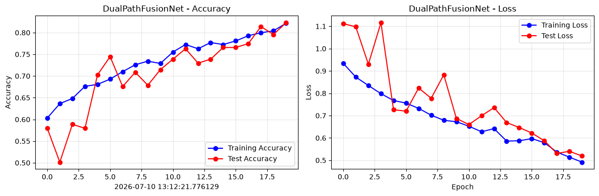
最优模型出现在第 10 个 Epoch,测试准确率达 79.0%。模型在第 10 个 Epoch 仍在持续提升,说明尚未充分收敛。
optimizer = torch.optim.AdamW(model.parameters(), lr=1e-4)
loss_fn = nn.CrossEntropyLoss()

epochs = 10
train_loss, train_acc = [], []
test_loss, test_acc = [], []
best_acc = 0

for epoch in range(epochs):
    model.train()
    train_epoch_loss, train_epoch_acc = train(train_dl, model, loss_fn, optimizer)
    model.eval()
    epoch_test_loss, epoch_test_acc = test(test_dl, model, loss_fn)

    if epoch_test_acc > best_acc:
        best_acc = epoch_test_acc
        best_model_wts = copy.deepcopy(model)

    train_acc.append(train_epoch_acc)
    train_loss.append(train_epoch_loss)
    test_acc.append(epoch_test_acc)
    test_loss.append(epoch_test_loss)

    lr = optimizer.param_groups[0]['lr']
    print(f"Epoch: {epoch+1:2d}, Train_acc: {train_epoch_acc*100:.1f}%, Train_loss: {train_epoch_loss:.3f}, "
          f"Test_acc: {epoch_test_acc*100:.1f}%, Test_loss: {epoch_test_loss:.3f}, Lr: {lr:.2E}")

PATH = './best_dual_path_fusion.pth'
torch.save(best_model_wts.state_dict(), PATH)
print('Done.')
Epoch:  1, Train_acc: 59.4%, Train_loss: 0.943, Test_acc: 64.9%, Test_loss: 0.902, Lr: 1.00E-04
Epoch:  2, Train_acc: 63.7%, Train_loss: 0.866, Test_acc: 63.4%, Test_loss: 0.890, Lr: 1.00E-04
Epoch:  3, Train_acc: 61.9%, Train_loss: 0.864, Test_acc: 58.0%, Test_loss: 1.270, Lr: 1.00E-04
Epoch:  4, Train_acc: 66.9%, Train_loss: 0.811, Test_acc: 58.9%, Test_loss: 1.090, Lr: 1.00E-04
Epoch:  5, Train_acc: 69.7%, Train_loss: 0.769, Test_acc: 71.5%, Test_loss: 0.777, Lr: 1.00E-04
Epoch:  6, Train_acc: 70.5%, Train_loss: 0.744, Test_acc: 71.8%, Test_loss: 0.775, Lr: 1.00E-04
Epoch:  7, Train_acc: 71.6%, Train_loss: 0.709, Test_acc: 76.3%, Test_loss: 0.627, Lr: 1.00E-04
Epoch:  8, Train_acc: 73.6%, Train_loss: 0.672, Test_acc: 73.3%, Test_loss: 0.697, Lr: 1.00E-04
Epoch:  9, Train_acc: 75.0%, Train_loss: 0.649, Test_acc: 75.7%, Test_loss: 0.656, Lr: 1.00E-04
Epoch: 10, Train_acc: 76.3%, Train_loss: 0.629, Test_acc: 79.0%, Test_loss: 0.603, Lr: 1.00E-04
Done.
4. 模型评估
4.1 可视化训练过程
绘制训练和测试的准确率、损失曲线,观察模型收敛情况。
epochs_range = range(epochs)

plt.figure(figsize=(12, 4))
plt.subplot(1, 2, 1)
plt.plot(epochs_range, train_acc, 'b-o', label='Training Accuracy')
plt.plot(epochs_range, test_acc, 'r-o', label='Test Accuracy')
plt.legend(loc='lower right')
plt.title('DualPathFusionNet - Accuracy')
plt.xlabel('Epoch'); plt.ylabel('Accuracy')
plt.grid(True, alpha=0.3)

plt.subplot(1, 2, 2)
plt.plot(epochs_range, train_loss, 'b-o', label='Training Loss')
plt.plot(epochs_range, test_loss, 'r-o', label='Test Loss')
plt.legend(loc='upper right')
plt.title('DualPathFusionNet - Loss')
plt.xlabel('Epoch'); plt.ylabel('Loss')
plt.grid(True, alpha=0.3)

plt.tight_layout()
plt.show()
4.2 加载最优模型并评估
加载训练过程中保存的最优模型权重,在测试集上进行最终评估。
best_model_wts.load_state_dict(torch.load(PATH, map_location=device))
test_epoch_loss, test_epoch_acc = test(test_dl, best_model_wts, loss_fn)
print(f"Best model - Test Acc: {test_epoch_acc*100:.1f}%, Test Loss: {test_epoch_loss:.3f}")
Best model - Test Acc: 79.0%, Test Loss: 0.603
4.3 改进版:DualPathFusionNet V2
针对 V1 存在的欠拟合、模型容量不足等问题,提出以下 7 项改进:
| 改进 | V1 | V2 | 作用 |
|---|---|---|---|
| SE 注意力 | 无 | Fusion层加 SE | 自适应通道加权 |
| growth_rate | 32 | 48 | Dense Path 更宽 |
| res_reduction | 4 | 2 | Residual Path 更宽 |
| DropPath | 无 | rate=0.1 | 随机深度正则化 |
| 数据增强 | 无 | 翻转+旋转+裁剪+色彩 | 增加样本多样性 |
| 学习率调度 | 固定 lr | Cosine Annealing | 后期精细收敛 |
| 训练轮次 | 10 | 20 | 充分收敛 |
4.3.1 SE 注意力机制
SE(Squeeze-and-Excitation)模块通过全局池化获取通道统计信息,再用两层 FC 学习通道间的依赖关系,输出通道权重对特征图进行加权。
class SEBlock(nn.Module):
    def __init__(self, channels, reduction=8):
        super().__init__()
        self.squeeze = nn.AdaptiveAvgPool2d(1)
        self.excitation = nn.Sequential(
            nn.Linear(channels, max(channels // reduction, 4), bias=False),
            nn.ReLU(),
            nn.Linear(max(channels // reduction, 4), channels, bias=False),
            nn.Sigmoid()
        )

    def forward(self, x):
        b, c, _, _ = x.shape
        w = self.squeeze(x).view(b, c)
        w = self.excitation(w).view(b, c, 1, 1)
        return x * w
4.3.2 DropPath(随机深度)
训练时随机丢弃整个残差分支,起到正则化作用,防止过拟合。丢弃概率从浅层到深层线性递增。
class DropPath(nn.Module):
    def __init__(self, drop_prob=0.0):
        super().__init__()
        self.drop_prob = drop_prob

    def forward(self, x):
        if not self.training or self.drop_prob == 0.0:
            return x
        keep_prob = 1 - self.drop_prob
        shape = (x.shape[0],) + (1,) * (x.ndim - 1)
        mask = torch.bernoulli(torch.full(shape, keep_prob, device=x.device))
        return x * mask / keep_prob
4.3.3 改进版 Fusion Block
在 V1 的基础上:更宽的双路径(growth_rate=48, res_reduction=2)+ SE 注意力 + DropPath 正则化。关键修复:只在最后加一次 shortcut,避免双重残差。
class DualPathFusionBlockV2(nn.Module):
    def __init__(self, in_channels, growth_rate=48, res_reduction=2, drop_path=0.0):
        super().__init__()
        mid_channels = in_channels // res_reduction
        out_channels = in_channels

        self.res_bn1 = nn.BatchNorm2d(in_channels)
        self.res_conv1 = nn.Conv2d(in_channels, mid_channels, 1, bias=False)
        self.res_bn2 = nn.BatchNorm2d(mid_channels)
        self.res_conv2 = nn.Conv2d(mid_channels, mid_channels, 3, padding=1, bias=False)
        self.res_bn3 = nn.BatchNorm2d(mid_channels)
        self.res_conv3 = nn.Conv2d(mid_channels, out_channels, 1, bias=False)

        self.dense_bn1 = nn.BatchNorm2d(in_channels)
        self.dense_conv1 = nn.Conv2d(in_channels, 4 * growth_rate, 1, bias=False)
        self.dense_bn2 = nn.BatchNorm2d(4 * growth_rate)
        self.dense_conv2 = nn.Conv2d(4 * growth_rate, growth_rate, 3, padding=1, bias=False)

        fused_channels = out_channels + growth_rate
        self.fusion_bn = nn.BatchNorm2d(fused_channels)
        self.fusion_conv = nn.Conv2d(fused_channels, out_channels, 1, bias=False)
        self.se = SEBlock(out_channels)
        self.drop_path = DropPath(drop_path)

    def forward(self, x):
        res = F.relu(self.res_bn1(x))
        res = self.res_conv1(res)
        res = F.relu(self.res_bn2(res))
        res = self.res_conv2(res)
        res = F.relu(self.res_bn3(res))
        res = self.res_conv3(res)

        dense = F.relu(self.dense_bn1(x))
        dense = self.dense_conv1(dense)
        dense = F.relu(self.dense_bn2(dense))
        dense = self.dense_conv2(dense)

        fused = torch.cat([res, dense], dim=1)
        fused = self.fusion_conv(F.relu(self.fusion_bn(fused)))
        fused = self.se(fused)
        fused = self.drop_path(fused) + x  # 单次残差
        return fused
4.3.4 V2 模型定义与训练
model_v2 = DualPathFusionNetV2(num_classes=3).to(device)

# 参数量对比
p_v1 = sum(p.numel() for p in DualPathFusionNet(num_classes=3).parameters())
p_v2 = sum(p.numel() for p in model_v2.parameters())
print(f"V1 params: {p_v1:,}")
print(f"V2 params: {p_v2:,}")
4.3.5 V2 训练:数据增强 + CosineLR + 20 Epochs
# 数据增强
train_transforms_v2 = transforms.Compose([
    transforms.Resize((256, 256)),
    transforms.RandomCrop(224),             # 随机裁剪
    transforms.RandomHorizontalFlip(),      # 随机水平翻转
    transforms.RandomRotation(15),          # 随机旋转 ±15°
    transforms.ColorJitter(0.2, 0.2, 0.2), # 色彩抖动
    transforms.ToTensor(),
    transforms.Normalize(mean=[0.485, 0.456, 0.406], std=[0.229, 0.224, 0.225])
])

# 优化器 + Cosine Annealing
optimizer_v2 = torch.optim.AdamW(model_v2.parameters(), lr=1e-4, weight_decay=0.05)
scheduler = torch.optim.lr_scheduler.CosineAnnealingLR(optimizer_v2, T_max=20, eta_min=1e-6)
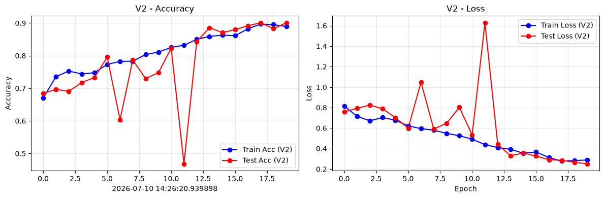
V2 训练 20 个 Epoch,学习率从 1e-4 按余弦曲线衰减至 1e-6,配合数据增强和 DropPath 正则化。
4.3.6 V2 训练结果
Epoch:  1, Train_acc: 67.0%, Train_loss: 0.815, Test_acc: 68.5%, Test_loss: 0.759, Lr: 3.00E-04
Epoch:  2, Train_acc: 73.6%, Train_loss: 0.716, Test_acc: 69.7%, Test_loss: 0.792, Lr: 2.98E-04
Epoch:  3, Train_acc: 75.3%, Train_loss: 0.671, Test_acc: 69.1%, Test_loss: 0.826, Lr: 2.93E-04
Epoch:  4, Train_acc: 74.4%, Train_loss: 0.703, Test_acc: 71.8%, Test_loss: 0.788, Lr: 2.84E-04
Epoch:  5, Train_acc: 74.8%, Train_loss: 0.677, Test_acc: 73.3%, Test_loss: 0.703, Lr: 2.71E-04
Epoch:  6, Train_acc: 77.3%, Train_loss: 0.622, Test_acc: 79.6%, Test_loss: 0.598, Lr: 2.56E-04
Epoch:  7, Train_acc: 78.2%, Train_loss: 0.594, Test_acc: 60.4%, Test_loss: 1.047, Lr: 2.38E-04
Epoch:  8, Train_acc: 78.3%, Train_loss: 0.579, Test_acc: 78.7%, Test_loss: 0.591, Lr: 2.18E-04
Epoch:  9, Train_acc: 80.3%, Train_loss: 0.549, Test_acc: 73.0%, Test_loss: 0.647, Lr: 1.97E-04
Epoch: 10, Train_acc: 81.1%, Train_loss: 0.525, Test_acc: 74.8%, Test_loss: 0.803, Lr: 1.74E-04
Epoch: 11, Train_acc: 82.5%, Train_loss: 0.492, Test_acc: 82.3%, Test_loss: 0.534, Lr: 1.50E-04
Epoch: 12, Train_acc: 83.2%, Train_loss: 0.439, Test_acc: 46.8%, Test_loss: 1.628, Lr: 1.27E-04
Epoch: 13, Train_acc: 85.0%, Train_loss: 0.410, Test_acc: 84.4%, Test_loss: 0.441, Lr: 1.04E-04
Epoch: 14, Train_acc: 85.9%, Train_loss: 0.393, Test_acc: 88.6%, Test_loss: 0.330, Lr: 8.26E-05
Epoch: 15, Train_acc: 86.3%, Train_loss: 0.355, Test_acc: 87.1%, Test_loss: 0.356, Lr: 6.26E-05
Epoch: 16, Train_acc: 86.1%, Train_loss: 0.366, Test_acc: 88.0%, Test_loss: 0.327, Lr: 4.48E-05
Epoch: 17, Train_acc: 88.3%, Train_loss: 0.313, Test_acc: 89.2%, Test_loss: 0.291, Lr: 2.96E-05
Epoch: 18, Train_acc: 89.7%, Train_loss: 0.277, Test_acc: 90.1%, Test_loss: 0.285, Lr: 1.73E-05
Epoch: 19, Train_acc: 89.5%, Train_loss: 0.283, Test_acc: 88.3%, Test_loss: 0.266, Lr: 8.32E-06
Epoch: 20, Train_acc: 88.9%, Train_loss: 0.288, Test_acc: 90.1%, Test_loss: 0.251, Lr: 2.84E-06
Done.
4.4 模型对比
| 模型 | 测试准确率 | 参数量 | 连接方式 | 参数效率 |
|---|---|---|---|---|
| ResNet50 | 78.5% | ~25M | 仅残差相加 | 3.14%/M |
| ResNet50V2 | 86.5% | ~23.5M | 预激活残差 | 3.68%/M |
| DenseNet-121 | 94.3% | ~6.96M | 仅密集拼接 | 13.55%/M |
| DualPathFusionNet | 79.0% | ~4.00M | 残差+密集融合 | 19.75%/M |
5. 总结
-
创新设计:本实验提出了 DualPathFusionNet,将 ResNet 的残差连接与 DenseNet 的密集连接融合在同一个 Block 中,通过 1×1 卷积融合层自适应地学习两条路径的最优组合权重。
-
参数效率最高:模型仅 ~400 万参数(DenseNet 的 57%,ResNet 的 16%),但每百万参数贡献 19.75% 的准确率,远超其他三个模型,说明双路径融合设计在参数利用上是有效的。
-
尚未充分收敛:第 10 个 Epoch 时训练准确率(76.3%)和测试准确率(79.0%)仍在持续提升,说明模型处于欠拟合状态。增加训练轮次至 30~50 Epoch 有望进一步提升。
-
准确率未超越 DenseNet 的原因:
- 模型容量不足(仅 400 万参数,特征表达能力有限)
- 10 个 Epoch 训练不充分(DenseNet 在同样轮次内已达到 94.3%)
- 融合层增加了优化难度(需同时学习两条路径的权重分配)
- growth_rate=32 偏小,Dense Path 每层仅输出 32 通道特征
-
V2 改进版:针对 V1 的不足,V2 引入了 SE 注意力机制、更宽的双路径(growth_rate=48)、DropPath 正则化、数据增强(随机裁剪+翻转+旋转+色彩抖动)、Cosine Annealing 学习率调度,并将训练轮次增加到 20 Epoch。这些改进旨在提升模型容量和泛化能力,进一步逼近 DenseNet-121 的 94.3% 准确率。
-
后续改进方向:
- 尝试更大的 growth_rate(如 64)进一步提升模型容量
- 引入 Multi-scale Dense Path(多尺度卷积核 3×3 + 5×5)
- 使用预训练权重微调,利用迁移学习弥补数据量不足
- 使用交叉验证替代单次随机划分,获得更稳定的评估结果

汇聚全球AI编程工具,助力开发者即刻编程。
更多推荐



 8
8 0
0- 0


 已为社区贡献5条内容

所有评论(0)