
《机器学习经典算法实战指南 —— 从KNN原理到手写数字识别完整项目》
前言
KNN 是机器学习领域中最简单、最直观的算法之一,常被誉为 “机器学习界的Hello World”。它的核心思想朴素得令人惊讶:“近朱者赤,近墨者黑” —— 想知道一个人是什么样的人,看看他身边最近的朋友就知道了。正是这种基于“相似性”的直觉,让 KNN 既能解决分类问题,也能处理回归问题,且在众多实际场景中表现不俗。
KNN算法
KNN算法简介
KNN算法思想
K-近邻算法(K Nearest Neighbor,简称KNN)。比如:根据你的“邻居”来推断出你的类别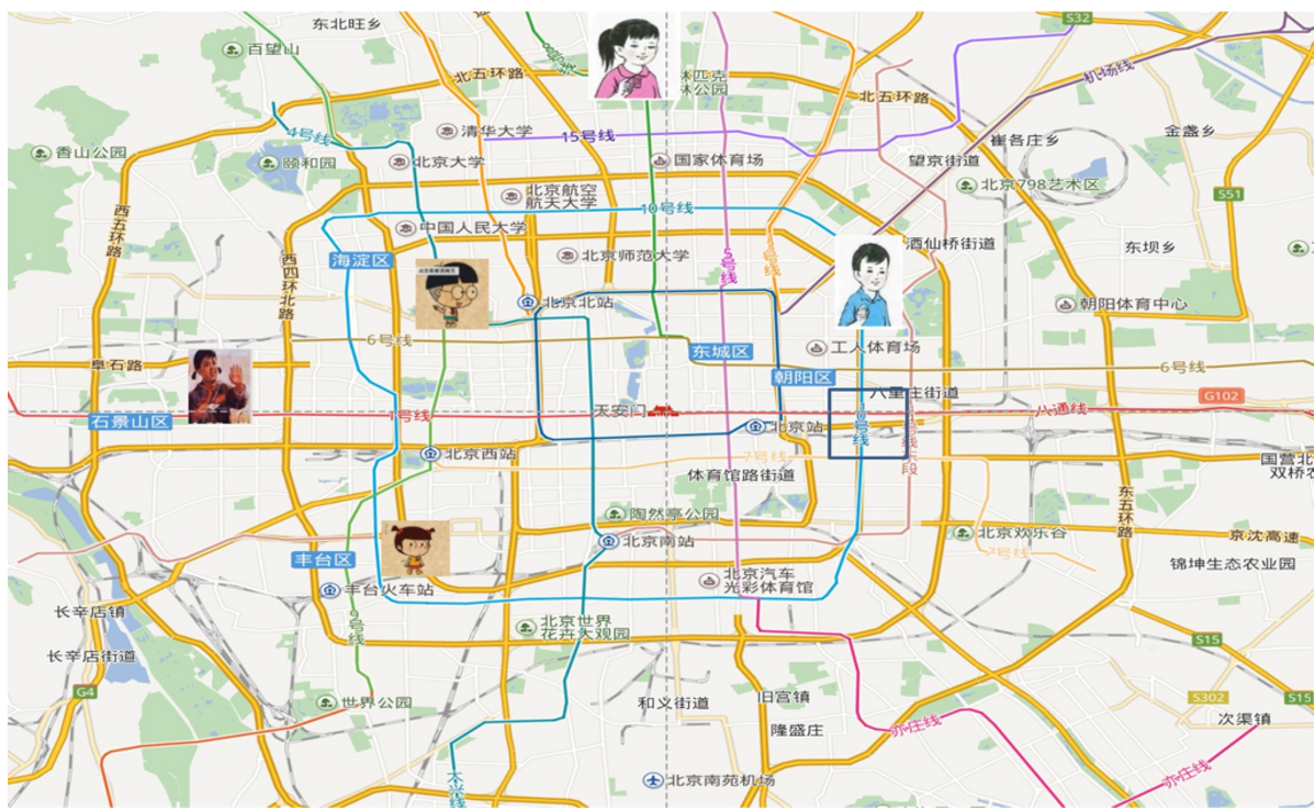
KNN算法思想:如果一个样本在特征空间中的 k 个最相似的样本中的大多数属于某一个类别,则该样本也属于这个类别
样本相似性:样本都是属于一个任务数据集的。样本距离越近则越相似。
利用K近邻算法预测电影类型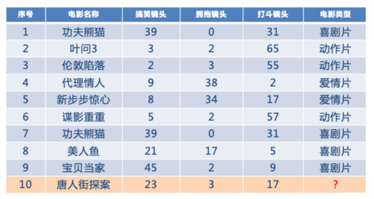
K值的选择
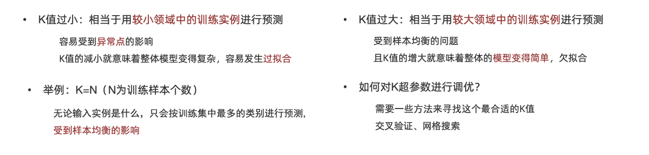
KNN的应用方式
解决问题:分类问题、回归问题
法思想:若一个样本在特征空间中的 k 个最相似的样本大多数属于某一个类别,则该样本也属于这个类别
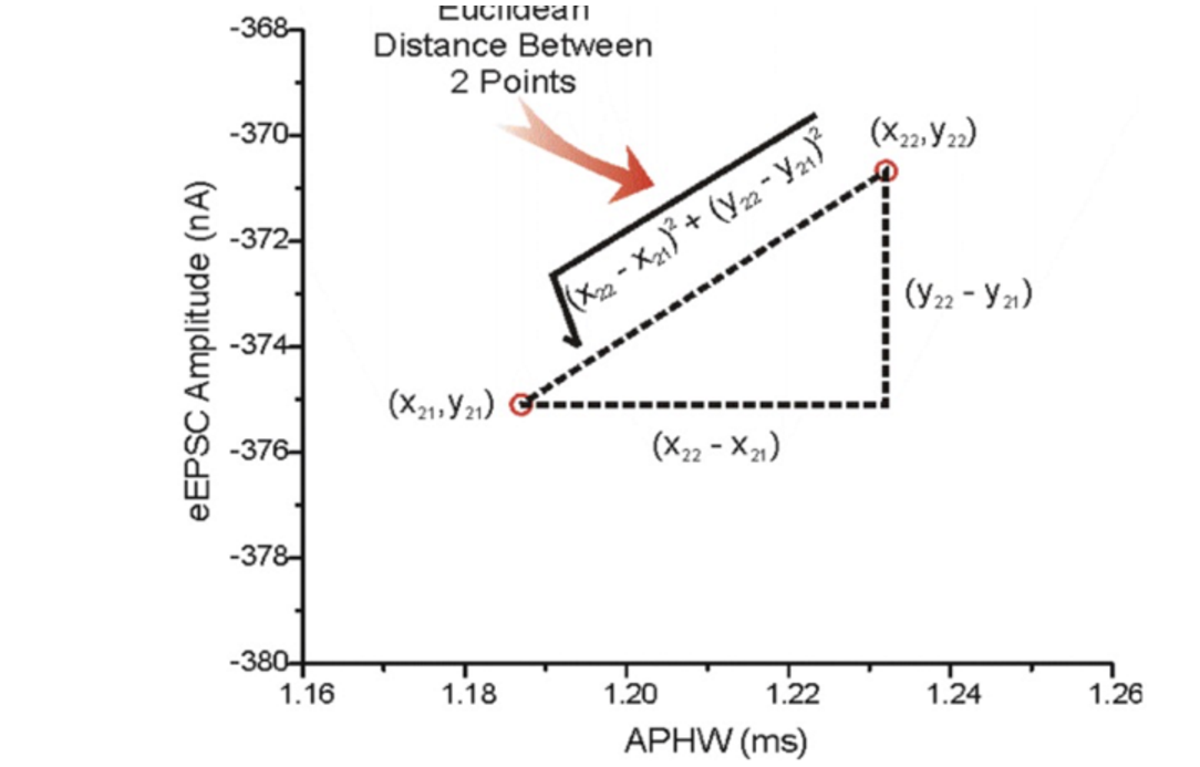
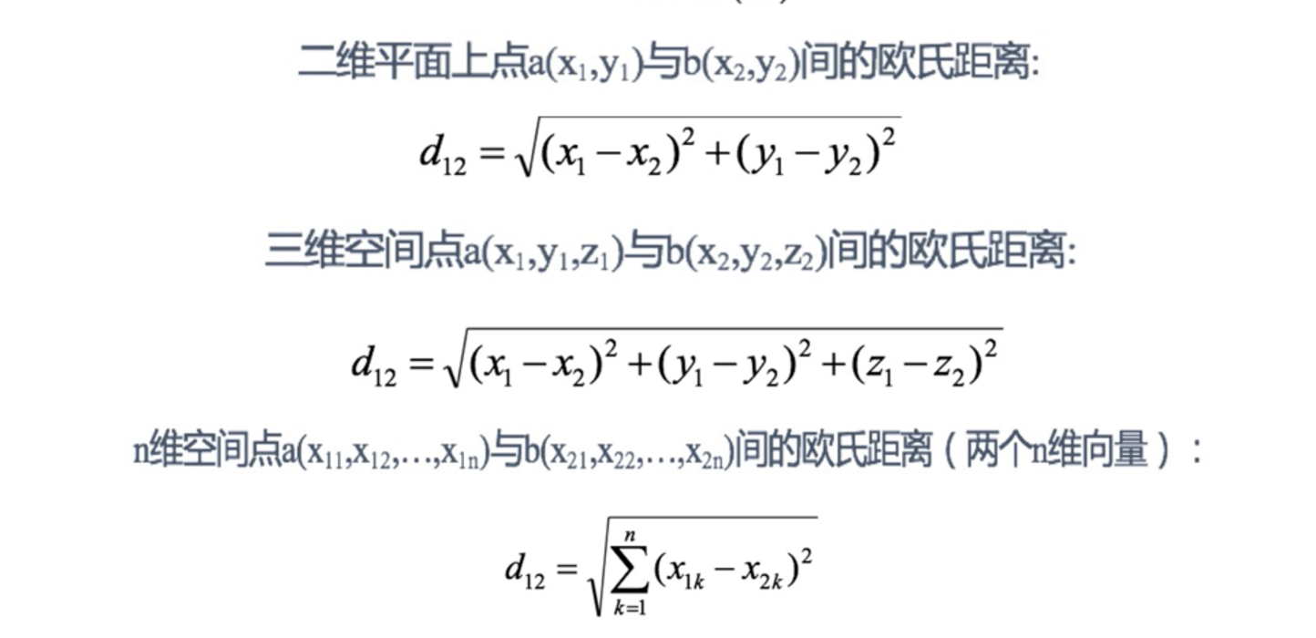
相似性:欧氏距离
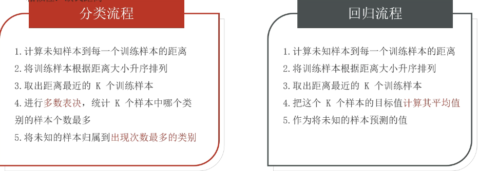
分类问题的处理流程:
- 计算未知样本到每一个训练样本的距离
- 将训练样本根据距离大小升序排列
- 取出距离最近的 K 个训练样本
- 进行多数表决,统计 K 个样本中哪个类别的样本个数最多
- 将未知的样本归属到出现次数最多的类别
回归问题的处理流程:
- 计算未知样本到每一个训练样本的距离
- 将训练样本根据距离大小升序排列
- 取出距离最近的 K 个训练样本
- 把这个 K 个样本的目标值计算其平均值
- 作为将未知的样本预测的值
API介绍
分类API
KNN分类API:
sklearn.neighbors.KNeighborsClassifier(n_neighbors=5)
n_neighbors:int,可选(默认= 5),k_neighbors查询默认使用的邻居数
#工具包
from sklearn.neighbors import KNeighborsClassifier,KNeighborsRegressor

x_train = [[0],[1],[4],[10],[8],[7]] # 训练集的特征
y_train = [0,0,1,1,1,0]  # 训练集的标签数据

x_test = [[5]]

#常见分类模型对象
model = KNeighborsClassifier(n_neighbors=3)

#模型训练
model.fit(x_train,y_train)

#模型预测
y_pred = model.predict(x_test)

print(f"预测值为:{y_pred}")
计算到所有训练样本的距离(欧氏距离):
|5-0| = 5(标签 0)
|5-1| = 4(标签 0)
|5-4| = 1(标签 1)
|5-10| = 5(标签 1)
|5-8| = 3(标签 1)
|5-7| = 2(标签 0)
按距离从小到大排序:
距离 1 → 特征 4,标签 1
距离 2 → 特征 7,标签 0
距离 3 → 特征 8,标签 1
距离 4 → 特征 1,标签 0
距离 5 → 特征 0(标签 0)和 10(标签 1)并列
取最近的 3 个邻居(距离 1, 2, 3):
标签 1 出现 2 次(来自特征 4 和 8)
标签 0 出现 1 次(来自特征 7)
多数投票:标签 1 票数多,所以预测结果为 1。
回归API
KNN回归API:
sklearn.neighbors.KNeighborsRegressor(n_neighbors=5)
# 工具包
from sklearn.neighbors import KNeighborsClassifier,KNeighborsRegressor

x_train = [[0,0,1],[1,1,0],[3,9,10],[4,8,12]]
y_train = [0.1,0.2,0.3,0.4]


model = KNeighborsRegressor(n_neighbors=2)

model.fit(x_train,y_train)

x_test = [[1,5,10]]

result = model.predict(x_test)

print(f"模型预测的数据为:{result}")
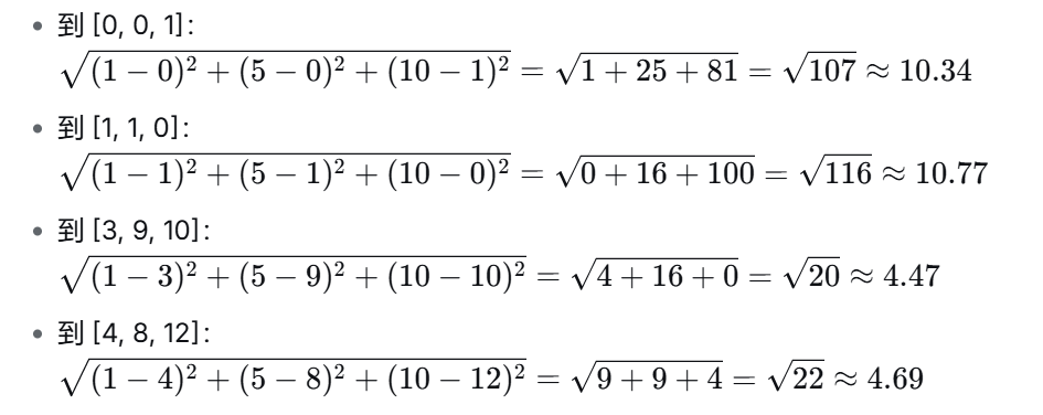
按距离从小到大:
[3, 9, 10] – 距离 ≈ 4.47,标签 0.3
[4, 8, 12] – 距离 ≈ 4.69,标签 0.4
[0, 0, 1] – 距离 ≈ 10.34
[1, 1, 0] – 距离 ≈ 10.77
最近的 2 个邻居是 前两个
KNeighborsRegressor 默认使用均值(weights=‘uniform’),即取两个邻居标签的平均值:

距离度量
欧式距离
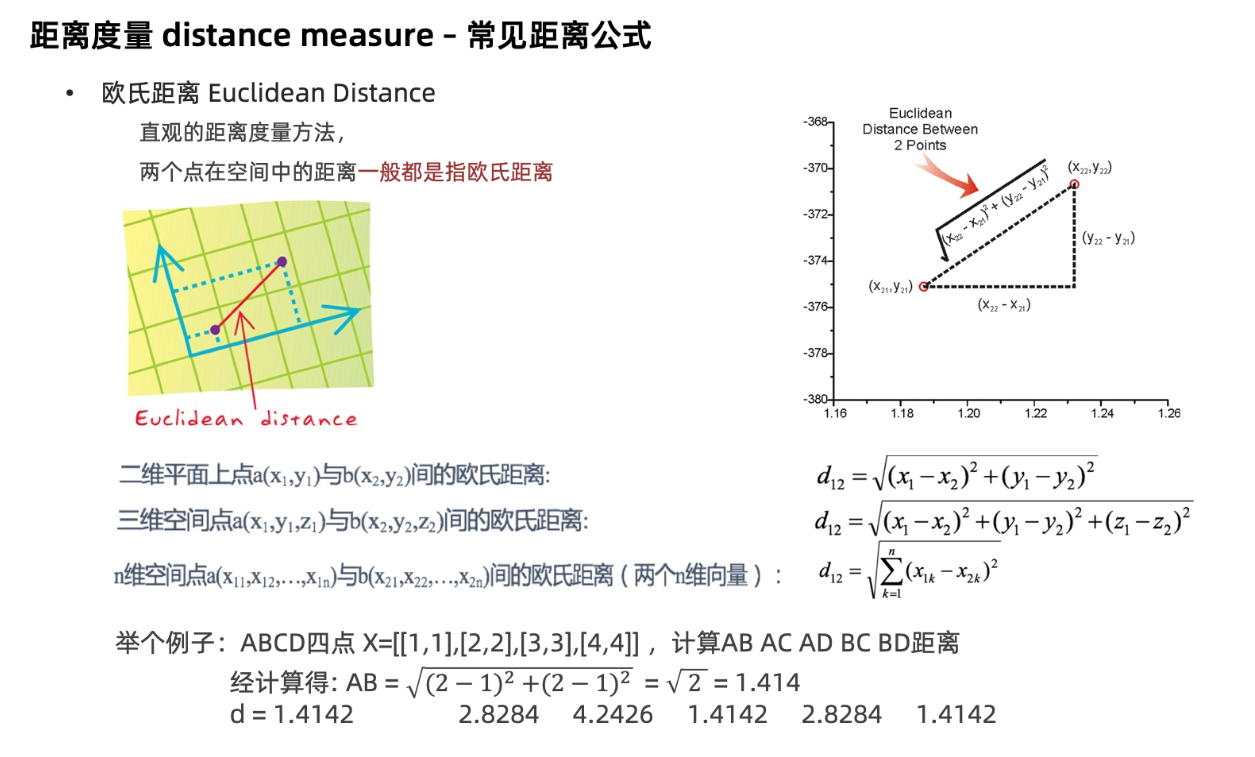
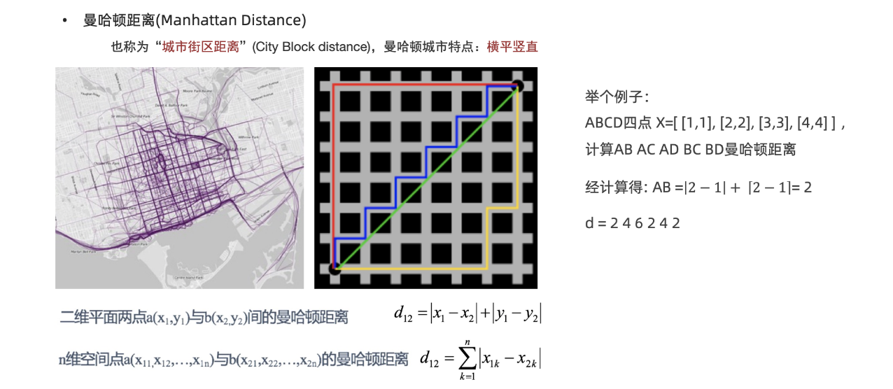
曼哈顿距离
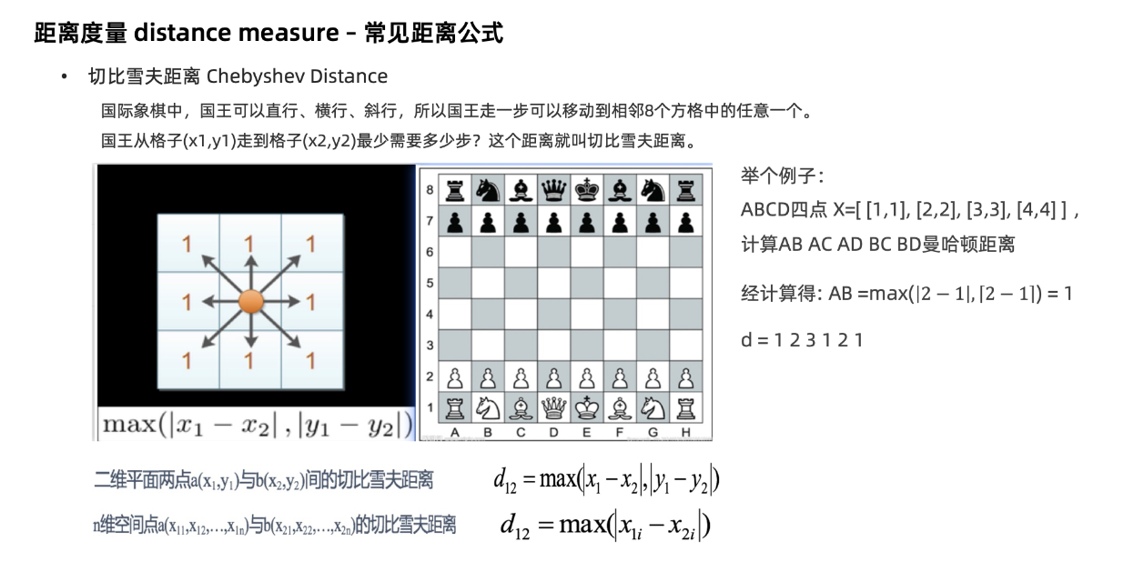
切比雪夫距离
闵氏距离
闵可夫斯基距离 Minkowski Distance 闵氏距离,不是一种新的距离的度量方式。而是距离的组合 是对多个距离度量公式的概括性的表述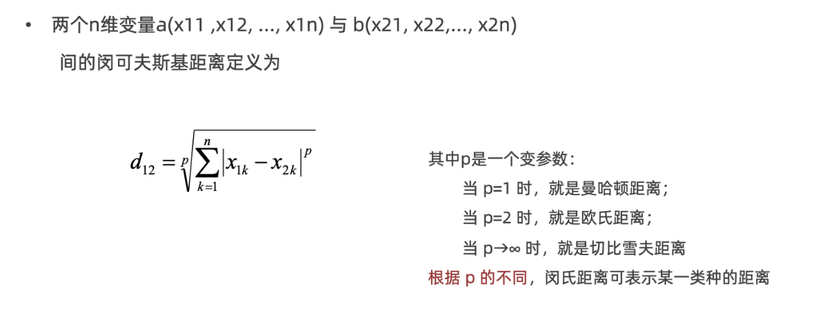
特征预处理
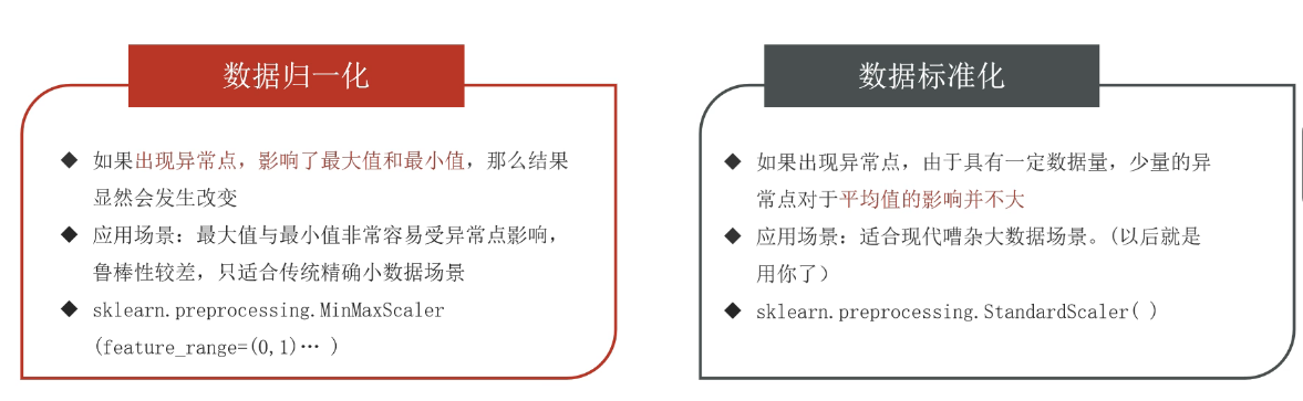
特征的单位或者大小相差较大,或者某特征的方差相比其他的特征要大出几个数量级,容易影响(支配)目标结果,使得一些模型(算法)无法学习到其它的特征。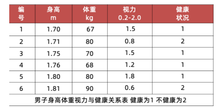
归一化
通过对原始数据进行变换把数据映射到【mi,mx】(默认为[0,1])之间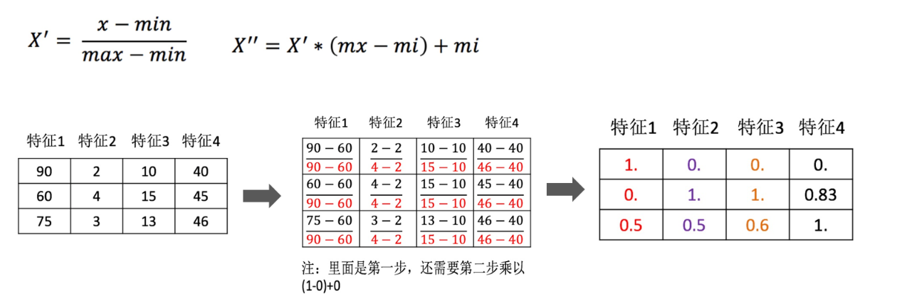
数据归一化的API实现
sklearn.preprocessing.MinMaxScaler (feature_range=(0,1)… )
feature_range 缩放区间
- 调用 fit_transform(X) 将特征进行归一化缩放
归一化受到最大值与最小值的影响,这种方法容易受到异常数据的影响, 鲁棒性较差,适合传统精确小数据场景
from sklearn.preprocessing import MinMaxScaler # 归一化对象

x_train = [
    [90,2,10,40],
    [60,4,15,45],
    [75,3,13,46]
]

# 创建归一化对象
scaler = MinMaxScaler()

# 对原数据集进行归一化操作
x_train_new = scaler.fit_transform(x_train)

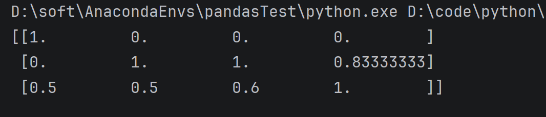
print(x_train_new)
标准化
通过对原始数据进行标准化,转换为均值为0标准差为1的标准正态分布的数据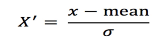
- mean 为特征的平均值
- σ 为特征的标准差
数据标准化的API实现
sklearn.preprocessing. StandardScaler()
调用 fit_transform(X) 将特征进行归一化缩放
# 1.导入工具包
from sklearn.preprocessing import MinMaxScaler,StandardScaler

# 2.数据(只有特征)
x_train = [[90, 2, 10, 40], [60, 4, 15, 45], [75, 3, 13, 46]]

# 3.实例化(归一化,标准化)
process =StandardScaler()

# 4.fit_transform 处理1
x_train_new =process.fit_transform(x_train)
print("标准化后的数据:\n")
print(x_train_new)

print("每个特征的均值:\n")
print(process.mean_)
print("每个特征的方差:\n")
print(process.var_)
print("每个特征的标准差:\n")
print(process.scale_)
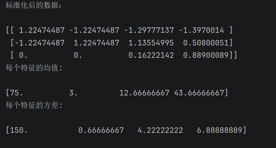
标准化的公式为:Z = (x - mean) / std(其中 std 是标准差,等于方差的平方根)。
StandardScaler 默认除以的是总体标准差(分母为 n,而非 n-1)。
让我们按列(特征) 分别计算:
第1列数据:[90, 60, 75]
均值 (mean):(90+60+75) / 3 = 75
方差 (var):[(90-75)² + (60-75)² + (75-75)²] / 3 = (225+225+0)/3 = 150
标准差 (std):√150 ≈ 12.247
转换结果:
90 → (90-75) / 12.247 ≈ 1.2247
60 → (60-75) / 12.247 ≈ -1.2247
75 → (75-75) / 12.247 = 0
第2列数据:[2, 4, 3]
均值:3
方差:[(2-3)² + (4-3)² + (3-3)²] / 3 = (1+1+0)/3 ≈ 0.6667
标准差:√0.6667 ≈ 0.8165
转换结果:
2 → (2-3) / 0.8165 ≈ -1.2247
4 → (4-3) / 0.8165 ≈ 1.2247
3 → 0
第3列数据:[10, 15, 13]
均值:(10+15+13)/3 ≈ 12.6667
方差:[(10-12.67)² + (15-12.67)² + (13-12.67)²] / 3 ≈ 4.2222
标准差:≈ 2.0548
第4列数据:[40, 45, 46]
均值:(40+45+46)/3 ≈ 43.6667
方差:[(40-43.67)² + (45-43.67)² + (46-43.67)²] / 3 ≈ 6.8889
利用KNN算法对鸢尾花分类
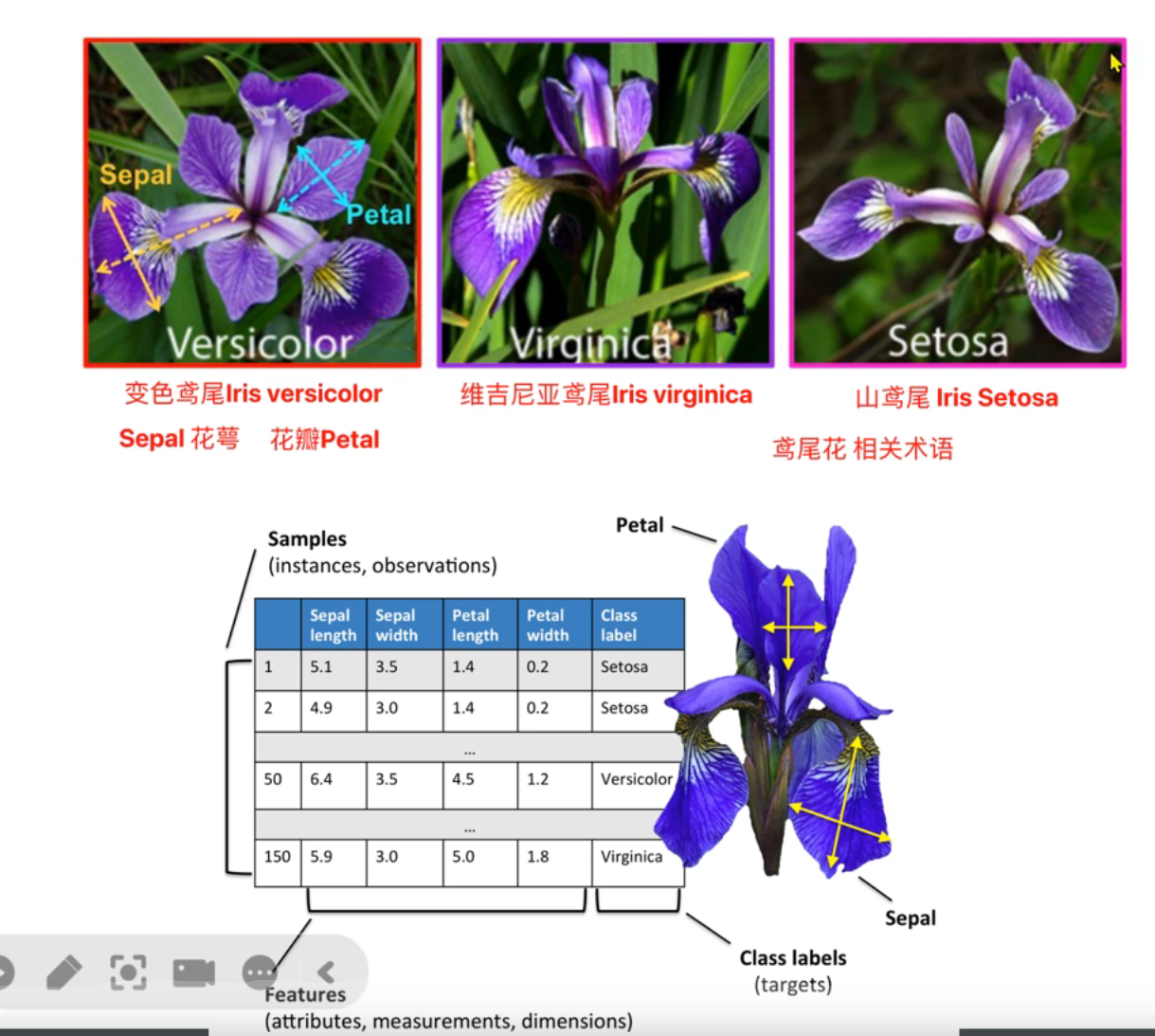
实现流程:
- 获取数据集
- 数据基本处理
- 数据集预处理-数据标准化
- 机器学习(模型训练)
- 模型评估
- 模型预测
# 定义函数 加载鸢尾花数据集
def dm01_loadiris():
    # 加载鸢尾花数据集
    iris_data = load_iris()

    # 1.1 查看数据集
    print(iris_data.data[:5])
    # 1.2 查看目标值.
    print(iris_data.target)
    # 1.3 查看目标值名字.
    print(iris_data.target_names)
    # 1.4 查看特征名.
    print(iris_data.feature_names)
    # 1.5 查看数据集的描述信息.
    print(iris_data.DESCR)
    # 1.6 查看数据文件路径
    print(iris_data.filename)
[[5.1 3.5 1.4 0.2]
 [4.9 3.  1.4 0.2]
 [4.7 3.2 1.3 0.2]
 [4.6 3.1 1.5 0.2]
 [5.  3.6 1.4 0.2]]
[0 0 0 0 0 0 0 0 0 0 0 0 0 0 0 0 0 0 0 0 0 0 0 0 0 0 0 0 0 0 0 0 0 0 0 0 0
 0 0 0 0 0 0 0 0 0 0 0 0 0 1 1 1 1 1 1 1 1 1 1 1 1 1 1 1 1 1 1 1 1 1 1 1 1
 1 1 1 1 1 1 1 1 1 1 1 1 1 1 1 1 1 1 1 1 1 1 1 1 1 1 2 2 2 2 2 2 2 2 2 2 2
 2 2 2 2 2 2 2 2 2 2 2 2 2 2 2 2 2 2 2 2 2 2 2 2 2 2 2 2 2 2 2 2 2 2 2 2 2
 2 2]
['setosa' 'versicolor' 'virginica']
['sepal length (cm)', 'sepal width (cm)', 'petal length (cm)', 'petal width (cm)']
.. _iris_dataset:

Iris plants dataset
--------------------

**Data Set Characteristics:**

:Number of Instances: 150 (50 in each of three classes)
:Number of Attributes: 4 numeric, predictive attributes and the class
:Attribute Information:
    - sepal length in cm
    - sepal width in cm
    - petal length in cm
    - petal width in cm
    - class:
            - Iris-Setosa
            - Iris-Versicolour
            - Iris-Virginica

:Summary Statistics:

============== ==== ==== ======= ===== ====================
                Min  Max   Mean    SD   Class Correlation
============== ==== ==== ======= ===== ====================
sepal length:   4.3  7.9   5.84   0.83    0.7826
sepal width:    2.0  4.4   3.05   0.43   -0.4194
petal length:   1.0  6.9   3.76   1.76    0.9490  (high!)
petal width:    0.1  2.5   1.20   0.76    0.9565  (high!)
============== ==== ==== ======= ===== ====================

:Missing Attribute Values: None
:Class Distribution: 33.3% for each of 3 classes.
:Creator: R.A. Fisher
:Donor: Michael Marshall (MARSHALL%PLU@io.arc.nasa.gov)
:Date: July, 1988

The famous Iris database, first used by Sir R.A. Fisher. The dataset is taken
from Fisher's paper. Note that it's the same as in R, but not as in the UCI
Machine Learning Repository, which has two wrong data points.

This is perhaps the best known database to be found in the
pattern recognition literature.  Fisher's paper is a classic in the field and
is referenced frequently to this day.  (See Duda & Hart, for example.)  The
data set contains 3 classes of 50 instances each, where each class refers to a
type of iris plant.  One class is linearly separable from the other 2; the
latter are NOT linearly separable from each other.

.. dropdown:: References

  - Fisher, R.A. "The use of multiple measurements in taxonomic problems"
    Annual Eugenics, 7, Part II, 179-188 (1936); also in "Contributions to
    Mathematical Statistics" (John Wiley, NY, 1950).
  - Duda, R.O., & Hart, P.E. (1973) Pattern Classification and Scene Analysis.
    (Q327.D83) John Wiley & Sons.  ISBN 0-471-22361-1.  See page 218.
  - Dasarathy, B.V. (1980) "Nosing Around the Neighborhood: A New System
    Structure and Classification Rule for Recognition in Partially Exposed
    Environments".  IEEE Transactions on Pattern Analysis and Machine
    Intelligence, Vol. PAMI-2, No. 1, 67-71.
  - Gates, G.W. (1972) "The Reduced Nearest Neighbor Rule".  IEEE Transactions
    on Information Theory, May 1972, 431-433.
  - See also: 1988 MLC Proceedings, 54-64.  Cheeseman et al"s AUTOCLASS II
    conceptual clustering system finds 3 classes in the data.
  - Many, many more ...

iris.csv
# 2. 定义函数 dm02_showiris(), 显示鸢尾花数据.
def dm02_showiris():
    # 1. 加载数据集, 查看数据
    iris_data = load_iris()
    # 2. 数据展示
    # 读取数据, 并设置 特征名为列名.
    iris_df = pd.DataFrame(iris_data.data, columns=iris_data.feature_names)
    # print(iris_df.head(5))
    iris_df['label'] = iris_data.target

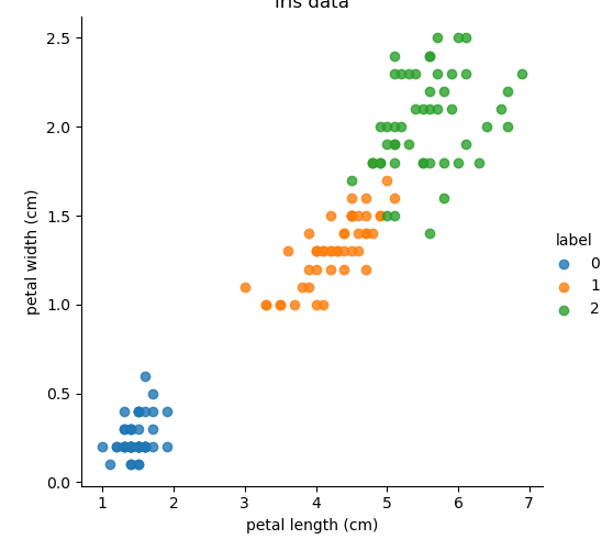
    # 可视化, x=花瓣长度, y=花瓣宽度, data=iris的df对象, hue=颜色区分, fit_reg=False 不绘制拟合回归线.
    sns.lmplot(x='petal length (cm)', y='petal width (cm)', data=iris_df, hue='label', fit_reg=False)
    plt.title('iris data')
    plt.show()
# 3. 定义函数 dm03_train_test_split(), 实现: 数据集划分
def dm03_train_test_split():
    # 1. 加载数据集, 查看数据
    iris_data = load_iris()
    # 2. 划分数据集, 即: 特征工程(预处理-标准化)
    x_train, x_test, y_train, y_test = train_test_split(iris_data.data, iris_data.target, test_size=0.2,
                                                        random_state=22)
    print(f'数据总数量: {len(iris_data.data)}')
    print(f'训练集中的x-特征值: {len(x_train)}')
    print(f'训练集中的y-目标值: {len(y_train)}')
    print(f'测试集中的x-特征值: {len(x_test)}')
iris_data.data(第一个参数)
含义:特征矩阵(自变量,X)。
这里是鸢尾花的 4 个物理特征(花萼长宽、花瓣长宽)。
iris_data.target(第二个参数)
含义:标签向量(因变量,y)。
这里是鸢尾花的 3 个类别(0, 1, 2)。
注意:这两个参数必须行数一致(即样本数量相同),函数会按相同索引进行配对拆分。
test_size=0.2
含义:测试集所占的比例(或绝对数量)。
这里 0.2 代表 20% 的数据划给测试集,剩下的 80%(1 - 0.2)自动划给训练集。
变形用法:如果你想指定具体数量,可以传整数,例如 test_size=30(表示测试集拿 30 个样本)。
random_state=22
含义:随机种子(Random Seed)。
拆分数据本质是“打乱(Shuffle)”后再切分。random_state=22 相当于给打乱算法设定了一个“固定起始点”。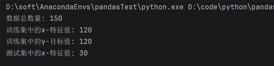
# 4. 定义函数 dm04_模型训练和预测(), 实现: 模型训练和预测
def dm04_model_train_and_predict():
    # 1. 加载数据集, 查看数据
    iris_data = load_iris()

    # 2. 划分数据集, 即: 数据基本处理
    x_train, x_test, y_train, y_test = train_test_split(iris_data.data, iris_data.target, test_size=0.2, random_state=22)

    # 3. 数据集预处理-数据标准化(即: 标准的正态分布的数据集)
    transfer = StandardScaler()
    # fit_transform(): 适用于首次对数据进行标准化处理的情况,通常用于训练集, 能同时完成 fit() 和 transform()。
    x_train = transfer.fit_transform(x_train)
    # transform(): 适用于对测试集进行标准化处理的情况,通常用于测试集或新的数据. 不需要重新计算统计量。
    x_test = transfer.transform(x_test)

    # 4. 机器学习(模型训练)
    estimator = KNeighborsClassifier(n_neighbors=5)
    estimator.fit(x_train, y_train)

    # 5. 模型评估.
    # 场景1: 对抽取出的测试集做预测.
    # 5.1 模型评估, 对抽取出的测试集做预测.
    y_predict = estimator.predict(x_test)
    print(f'预测结果为: {y_predict}')

    # 场景2: 对新的数据进行预测.
    # 5.2 模型预测, 对测试集进行预测.
    # 5.2.1 定义测试数据集.
    my_data = [[5.1, 3.5, 1.4, 0.2]]
    # 5.2.2 对测试数据进行-数据标准化.
    my_data = transfer.transform(my_data)
    # 5.2.3 模型预测.
    my_predict = estimator.predict(my_data)
    print(f'预测结果为: {my_predict}')

    # 5.2.4 模型预测概率, 返回每个类别的预测概率
    my_predict_proba = estimator.predict_proba(my_data)
    print(f'预测概率为: {my_predict_proba}')

    # 6. 模型预估, 有两种方式, 均可.
    # 6.1 模型预估, 方式1: 直接计算准确率, 100个样本中模型预测正确的个数.
    my_score = estimator.score(x_test, y_test)
    print(my_score)

    # 6.2 模型预估, 方式2: 采用预测值和真实值进行对比, 得到准确率.
    print(accuracy_score(y_test, y_predict))
fit_transform() = “学习 + 应用”。它会先看完训练集的所有数据,计算出这组数据专属的均值(mean_)和方差(var_),然后用这套参数去转换数据。
transform() = “只应用,不学习”。它直接使用已经学好的那套均值方差去转换,绝不窥探新数据的整体分布。

超参数选择的方法
交叉验证
交叉验证是一种数据集的分割方法,将训练集划分为 n 份,其中一份做验证集、其他n-1份做训练集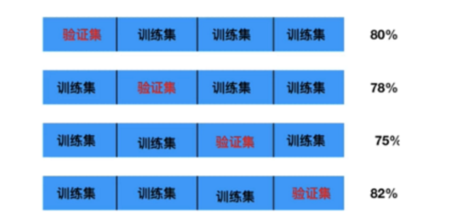
交叉验证法原理:将数据集划分为 cv=10 份:
- 第一次:把第一份数据做验证集,其他数据做训练
- 第二次:把第二份数据做验证集,其他数据做训练
- … 以此类推,总共训练10次,评估10次。
- 使用训练集+验证集多次评估模型,取平均值做交叉验证为模型得分
- 若k=5模型得分最好,再使用全部训练集(训练集+验证集) 对k=5模型再训练一边,再使用测试集对k=5模型做评估

网格搜索
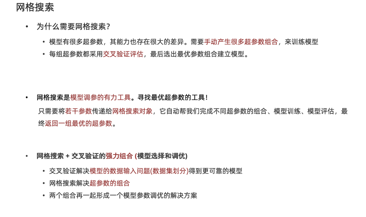
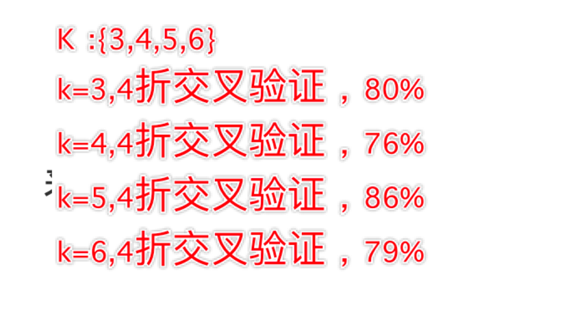
交叉验证网格搜索的API: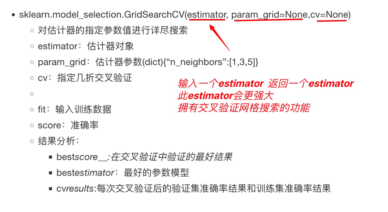
# 导入必要的工具包
from sklearn.datasets import load_iris   # 鸢尾花数据集
from sklearn.model_selection import train_test_split    # 分割训练集和测试集的
from sklearn.preprocessing import StandardScaler        # 数据标准化的
from sklearn.neighbors import KNeighborsClassifier      # KNN算法 分类对象
from sklearn.model_selection import GridSearchCV


# 获取数据
iris_data = load_iris()

# 数据基本处理
x_train, x_test, y_train, y_test = train_test_split(iris_data.data, iris_data.target, test_size=0.2, random_state=22)

# 数据集预处理 标准化
transfer = StandardScaler()
x_train = transfer.fit_transform(x_train)
x_test = transfer.transform(x_test)

# 模型训练
#  创建估计器对象
estimator = KNeighborsClassifier()
# 使用校验验证网格搜索 指定参数范围
param_dict = {"n_neighbors": range(1,10)}

# 具体的 网格搜索过程 + 交叉验证.
# 参1: 估计器对象, 参2: 参数范围, 参3: 交叉验证的折数.
estimator = GridSearchCV(estimator, param_grid=param_dict, cv=5)
# 具体的模型训练过程
estimator.fit(x_train, y_train)

# 交叉验证, 网格搜索结果查看.
print(estimator.best_score_)       # 模型在交叉验证中, 所有参数组合中的最高平均测试得分
print(estimator.best_estimator_)   # 最优的估计器对象.
print(estimator.cv_results_)       # 模型在交叉验证中的结果.
print(estimator.best_params_)      # 模型在交叉验证中的结果.

# 得到最优模型后, 对模型重新预测.
estimator = KNeighborsClassifier(n_neighbors=6)
estimator.fit(x_train, y_train)
print(f'模型评估: {estimator.score(x_test, y_test)}')   # 因为数据量和特征的问题, 该值可能小于上述的平均测试得分.
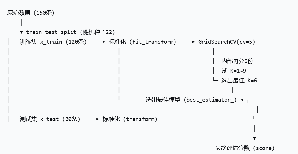
内部再拆分:它拿到 x_train(120 条数据)后,按照 cv=5,把这 120 条再平均切成 5 份(每份 24 条)。
循环打擂台(自动试 K 值):
第 1 轮:K=1。拿第 1 份(24条)当验证集,后 4 份(96条)当训练集,算出一个分数。
第 2 轮:K=1。拿第 2 份当验证集,其他当训练集,再算一个分数。
…(共 5 轮,算出 K=1 的平均分)
接着算 K=2 的 5 轮平均分,K=3 的 5 轮平均分……一直算到 K=9。
揭晓冠军:比较这 9 个平均分,谁最高就把谁记下来。
0.9666666666666666
KNeighborsClassifier(n_neighbors=6)
{'mean_fit_time': array([0.00087161, 0.00077167, 0.00075231, 0.00075827, 0.00073991,
       0.00077477, 0.00076561, 0.00077629, 0.00075746]), 'std_fit_time': array([1.39304399e-04, 3.26759078e-05, 3.06482794e-05, 3.95920164e-05,
       1.31434175e-05, 2.28502038e-05, 3.71322375e-05, 4.13236556e-05,
       4.10764146e-05]), 'mean_score_time': array([0.00164375, 0.00160966, 0.00161328, 0.00152478, 0.00150075,
       0.0015758 , 0.00153155, 0.00154238, 0.00154285]), 'std_score_time': array([2.16297330e-04, 1.91910672e-04, 1.13171712e-04, 7.61032104e-05,
       5.84773463e-05, 1.39913692e-04, 3.73581144e-05, 7.49163228e-05,
       6.42597827e-05]), 'param_n_neighbors': masked_array(data=[1, 2, 3, 4, 5, 6, 7, 8, 9],
             mask=[False, False, False, False, False, False, False, False,
                   False],
       fill_value=999999), 'params': [{'n_neighbors': 1}, {'n_neighbors': 2}, {'n_neighbors': 3}, {'n_neighbors': 4}, {'n_neighbors': 5}, {'n_neighbors': 6}, {'n_neighbors': 7}, {'n_neighbors': 8}, {'n_neighbors': 9}], 'split0_test_score': array([0.95833333, 0.95833333, 0.95833333, 1.        , 1.        ,
       1.        , 1.        , 1.        , 0.95833333]), 'split1_test_score': array([0.95833333, 0.91666667, 0.91666667, 0.95833333, 0.91666667,
       0.91666667, 0.91666667, 0.91666667, 0.91666667]), 'split2_test_score': array([0.95833333, 0.875     , 0.95833333, 0.95833333, 1.        ,
       1.        , 1.        , 1.        , 1.        ]), 'split3_test_score': array([0.875     , 0.875     , 0.875     , 0.875     , 0.91666667,
       0.95833333, 0.91666667, 0.91666667, 0.91666667]), 'split4_test_score': array([0.95833333, 0.95833333, 0.95833333, 0.91666667, 0.95833333,
       0.95833333, 0.95833333, 0.95833333, 0.95833333]), 'mean_test_score': array([0.94166667, 0.91666667, 0.93333333, 0.94166667, 0.95833333,
       0.96666667, 0.95833333, 0.95833333, 0.95      ]), 'std_test_score': array([0.03333333, 0.0372678 , 0.03333333, 0.04249183, 0.0372678 ,
       0.03118048, 0.0372678 , 0.0372678 , 0.03118048]), 'rank_test_score': array([7, 9, 8, 6, 2, 1, 2, 2, 5], dtype=int32)}
{'n_neighbors': 6}
模型评估: 0.9333333333333333
利用KNN算法实现手写数字识别
MNIST手写数字识别 是计算机视觉领域中 "hello world"级别的数据集
- 1999年发布,成为分类算法基准测试的基础
- 随着新的机器学习技术的出现,MNIST仍然是研究人员和学习者的可靠资源。
数据介绍
数据文件 train.csv 和 test.csv 包含从 0 到 9 的手绘数字的灰度图像。
- 每个图像高 28 像素,宽28 像素,共784个像素。
- 每个像素取值范围[0,255],取值越大意味着该像素颜色越深
- 训练数据集(train.csv)共785列。第一列为 “标签”,为该图片对应的手写数字。其余784列为该图像的像素值
- 训练集中的特征名称均有pixel前缀,后面的数字([0,783])代表了像素的序号。
像素组成图像如下: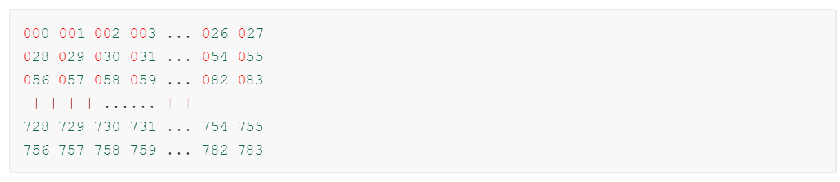
数据集示例如下: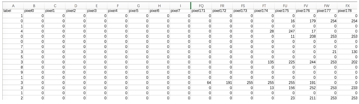
# 1. 显示图片.
def show_digit(idx):
    # 1.1 加载数据.
    data = pd.read_csv('../data/手写数字识别.csv')
    # 1.2非法值校验.
    if idx < 0 or idx > len(data) - 1:
        return
    # 1.3 打印数据基本信息
    x = data.iloc[:, 1:]
    y = data.iloc[:, 0]
    print(f'数据基本信息: {x.shape})')
    print(f'类别数据比例: {Counter(y)}')

    # 显示图片
    # 1.4 将数据形状修改为: 28*28
    digit = x.iloc[idx].values.reshape(28, 28)
    # 1.5 关闭坐标轴标签
    plt.axis('off')
    # 1.6 显示图像
    plt.imshow(digit, cmap='gray')  # 灰色显示
    plt.show()
iloc 用于按位置选取数据:
x:所有样本的特征(去掉第 0 列标签)。
y:所有样本的标签。
使用 Counter(y)(来自 collections 模块)统计每个数字(0~9)出现的频次,便于观察数据集类别分布。
从特征矩阵中取出第 idx 行(对应一个样本的 784 个像素值),将其转换为 numpy 数组,然后重塑为 28 行 × 28 列 的二维矩阵,以便用图像方式展示。
idx = 0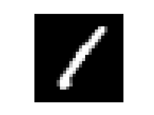
# 2. 训练模型.
def train_model():
    # 1. 加载数据.
    data = pd.read_csv('手写数字识别.csv')
    x = data.iloc[:, 1:]
    y = data.iloc[:, 0]

    # 2.数据预处理, 归一化.
    x = x / 255

    # 3. 分割训练集和测试集.
    # stratify: 按照y的类别比例进行分割
    x_train, x_test, y_train, y_test = train_test_split(x, y, test_size=0.2, stratify=y, random_state=21)

    # 4. 训练模型
    estimator = KNeighborsClassifier(n_neighbors=3)
    estimator.fit(x_train, y_train)

    # 5. 模型评估
    my_score = estimator.score(x_test, y_test)
    print(f'测试集准确率为: {my_score:.2f}')

    # 6. 模型保存.
    joblib.dump(estimator, '../data/knn.pth')
joblib 是 Python 中专门用于高效序列化大型 NumPy 对象的库(比 pickle 更快,特别是处理数组时)。
joblib.dump()代码将训练好的 KNN 模型(包含全部训练数据)保存到 …/data/knn.pth 文件中。

# 3. 测试模型.
def use_model():
    # 1. 读取图片
    img = plt.imread('../data/demo.png')   # 灰度图, 28*28像素
    plt.imshow(img, cmap='gray')
    plt.show()

    # 2. 加载模型.
    estimator = joblib.load('../data/knn.pth')

    # 3. 预测图片.
    img = img.reshape(1, -1)  # 形状从: (28, 28) => (1, 784)
    # print(img.shape)
    y_test = estimator.predict(img)
    print(f'您绘制的数字是: {y_test}')
plt.imread():使用 Matplotlib 读取图片文件,返回一个 NumPy 数组。
因为图片是灰度图(单通道),读取后的数组形状为 (28, 28)。
plt.imshow() 和 plt.show():将数组以灰度图像形式显示出来,方便你肉眼确认图片内容
joblib.load() 读取之前用 joblib.dump() 保存的 KNN 模型文件。
模型对象内部已经保存了训练集的所有数据(用于计算距离),可以直接调用 .predict() 方法进行预测。
图片形状是 (28, 28),必须变成 (1, 784)(1 张图片,784 个特征)才能喂给模型。
-1 表示自动计算该维度大小,这里 28×28=784,所以写 (1, -1) 等价于 (1, 784)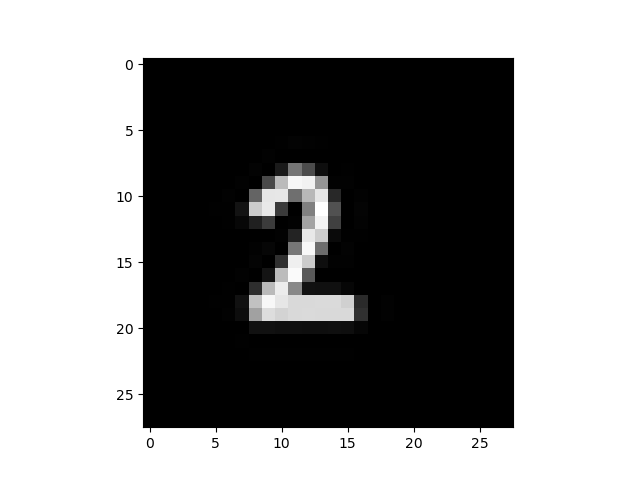

plt.imread() 读取 PNG 格式图片时,返回的像素值默认已经是 [0, 1] 的浮点数
总结
KNN 的魅力在于它的简单与强大共存 —— 它用最朴素的方式解释了机器学习的核心思想:数据决定结果,相似性衡量一切。它不需要复杂地模型假设,也不涉及深奥地数学推导,却能在实际应用中表现出色。
希望通过本文,你不仅学会了 KNN 的使用方法,更重要的是理解了机器学习项目的完整工作流:数据加载 → 探索性分析 → 特征预处理 → 模型训练与调优 → 模型保存与部署。这个流程是通用的,无论是 KNN 还是深度学习,都遵循这一基本范式。

汇聚全球AI编程工具,助力开发者即刻编程。
更多推荐



 11
11 0
0- 0


 已为社区贡献20条内容

所有评论(0)