从发现到定位的最后一公里：机器学习时序异常检测与根因分析结合实践

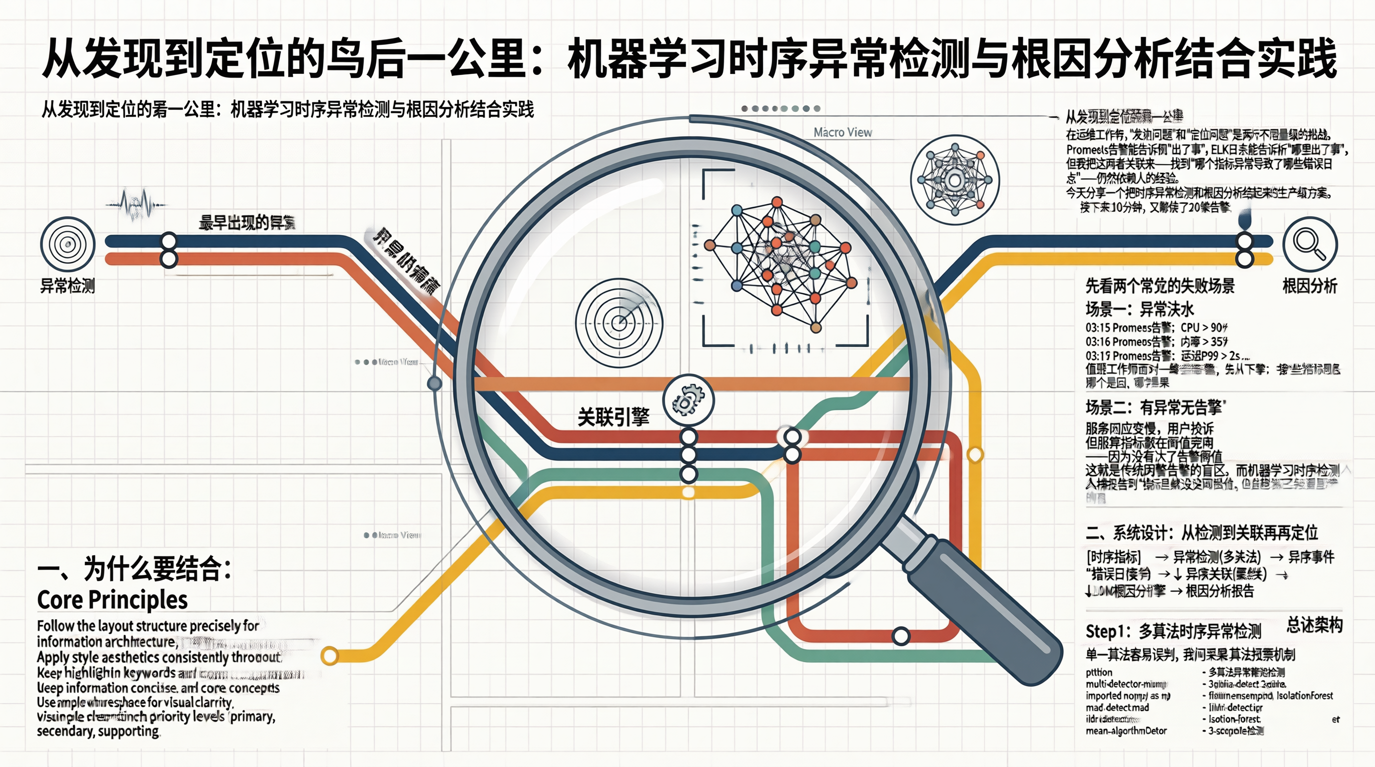
一、为什么要结合？

1.1 孤立的痛点

先看两个常见的失败场景：

场景一：异常洪水

03:15 Prometheus告警：CPU > 90%
03:16 Prometheus告警：内存 > 85%
03:17 Prometheus告警：磁盘IO > 95%
03:18 Prometheus告警：延迟P99 > 2s
... 接下来10分钟，又触发了20条告警

值班工程师面对一堆告警，无从下手。这些指标到底哪个是因、哪个是果？

场景二：有异常无告警

服务响应变慢，用户投诉
但所有指标都在阈值范围内
——因为没有达到告警阈值

这就是传统阈值告警的盲区。而机器学习时序检测可以捕捉到"指标虽然没超阈值，但趋势已经明显异常"的情况。

二、系统设计：从检测到关联再到定位

2.1 总体架构

flowchart TD
    A["[时序指标]"] --> B["异常检测(多算法)"] --> C["异常事件"]
    D["[错误日志]"] --> E["错误聚合(聚类)"] --> F["错误模式"]
    C --> G["异常关联引擎"]
    F --> G
    G --> H["LLM根因分析器"] --> I["根因分析报告"]

2.2 多算法时序异常检测

单一算法容易误判，我们采用多算法投票机制：

# multi_detector.py — 多算法异常检测
import numpy as np
from scipy import stats
from sklearn.ensemble import IsolationForest
import pandas as pd

class MultiAlgorithmDetector:
    """多算法异常检测引擎"""
    
    def __init__(self):
        self.detectors = {
            '3sigma': self._detect_3sigma,
            'mad': self._detect_mad,
            'iqr': self._detect_iqr,
            'isolation_forest': self._detect_iforest
        }
    
    def _detect_3sigma(self, series: pd.Series):
        """3-sigma检测"""
        mean = series.mean()
        std = series.std()
        anomalies = (series > mean + 3*std) | (series < mean - 3*std)
        return anomalies, mean, std
    
    def _detect_mad(self, series: pd.Series):
        """MAD（中位数绝对偏差）检测，对异常值更鲁棒"""
        median = series.median()
        mad = np.median(np.abs(series - median))
        # 阈值：median ± 3 * 1.4826 * MAD
        threshold = 3 * 1.4826 * mad
        anomalies = (series > median + threshold) | (series < median - threshold)
        return anomalies, median, threshold
    
    def _detect_iqr(self, series: pd.Series):
        """IQR四分位距检测"""
        q1 = series.quantile(0.25)
        q3 = series.quantile(0.75)
        iqr = q3 - q1
        lower = q1 - 1.5 * iqr
        upper = q3 + 1.5 * iqr
        anomalies = (series < lower) | (series > upper)
        return anomalies, lower, upper
    
    def _detect_iforest(self, series: pd.Series):
        """Isolation Forest检测"""
        values = series.values.reshape(-1, 1)
        model = IsolationForest(contamination=0.05, random_state=42)
        preds = model.fit_predict(values)
        anomalies = pd.Series(preds == -1, index=series.index)
        return anomalies, None, None
    
    def ensemble_detect(self, series: pd.Series, 
                        min_votes: int = 2):
        """集成投票：至少2个算法判定为异常才算异常"""
        votes = np.zeros(len(series))
        
        for name, detector in self.detectors.items():
            anomalies, _, _ = detector(series)
            votes += anomalies.astype(int)
        
        # 投票决定
        final_anomaly = votes >= min_votes
        anomaly_score = votes / len(self.detectors)
        
        return {
            'is_anomaly': final_anomaly,
            'confidence': anomaly_score,
            'votes': votes,
            'details': {name: detector(series)[0].tolist() 
                       for name, detector in self.detectors.items()}
        }

2.3 日志错误模式聚类

# log_cluster.py — 日志错误模式聚类
import re
from collections import Counter
from sklearn.feature_extraction.text import TfidfVectorizer
from sklearn.cluster import DBSCAN

class ErrorLogCluster:
    """错误日志模式聚类"""
    
    def __init__(self):
        self.patterns = {}
        self.vectorizer = TfidfVectorizer(
            analyzer='char_wb',
            ngram_range=(3, 5),
            max_features=1000
        )
    
    def normalize_log(self, message: str) -> str:
        """将变量部分替换为占位符"""
        # 替换IP地址
        message = re.sub(r'\d{1,3}\.\d{1,3}\.\d{1,3}\.\d{1,3}', '{ip}', message)
        # 替换数字
        message = re.sub(r'\d+', '{n}', message)
        # 替换UUID
        message = re.sub(r'[0-9a-f]{8}-[0-9a-f]{4}-[0-9a-f]{4}-[0-9a-f]{4}-[0-9a-f]{12}', 
                        '{uuid}', message)
        return message
    
    def cluster(self, log_entries: list) -> dict:
        """聚类错误日志"""
        messages = [entry['message'] for entry in log_entries]
        normalized = [self.normalize_log(m) for m in messages]
        
        # TF-IDF向量化 + DBSCAN聚类
        X = self.vectorizer.fit_transform(normalized)
        clustering = DBSCAN(eps=0.3, min_samples=2, metric='cosine')
        labels = clustering.fit_predict(X)
        
        # 统计每个聚类的数量和样本
        clusters = {}
        for i, label in enumerate(labels):
            if label == -1:
                continue  # 噪点忽略
            if label not in clusters:
                clusters[label] = {
                    'count': 0,
                    'pattern': normalized[i],
                    'sample_message': messages[i]
                }
            clusters[label]['count'] += 1
        
        # 按数量排序
        sorted_clusters = sorted(
            clusters.values(),
            key=lambda x: x['count'],
            reverse=True
        )
        
        return {
            'total_errors': len(log_entries),
            'clusters': sorted_clusters[:10],
            'unique_patterns': len(clusters)
        }

2.4 异常关联引擎

这是最关键的一步——把指标异常和日志错误关联起来：

# anomaly_correlator.py — 异常关联引擎
from datetime import datetime, timedelta
import numpy as np

class AnomalyCorrelator:
    """异常关联引擎：找到指标异常和日志错误的因果关系"""
    
    def __init__(self, time_window: int = 5):
        self.time_window = time_window  # 关联时间窗口（分钟）
    
    def correlate(self, metric_anomalies: dict, 
                  log_clusters: dict,
                  time_range: tuple) -> dict:
        """核心关联逻辑"""
        correlations = []
        
        # 对每个异常指标，检查同一时间窗口内的日志模式
        for metric_name, anomaly_info in metric_anomalies.items():
            anomaly_times = anomaly_info['anomaly_times']
            
            for atime in anomaly_times:
                window_start = atime - timedelta(minutes=self.time_window)
                window_end = atime + timedelta(minutes=self.time_window)
                
                # 找这个时间窗口内的错误日志
                matching_errors = [
                    c for c in log_clusters['clusters']
                    if any(window_start <= e['timestamp'] <= window_end 
                          for e in c.get('entries', []))
                ]
                
                if matching_errors:
                    correlations.append({
                        'metric': metric_name,
                        'anomaly_time': atime.isoformat(),
                        'anomaly_value': anomaly_info['value'],
                        'baseline': anomaly_info['baseline'],
                        'deviation': f"{((anomaly_info['value'] / anomaly_info['baseline']) - 1) * 100:.1f}%",
                        'related_errors': [
                            {
                                'pattern': c['pattern'],
                                'count': c['count'],
                                'sample': c['sample_message']
                            }
                            for c in matching_errors
                        ],
                        'correlation_strength': len(matching_errors) / len(log_clusters['clusters'])
                    })
        
        # 按关联强度排序
        correlations.sort(key=lambda x: x['correlation_strength'], reverse=True)
        
        return {
            'total_correlations': len(correlations),
            'top_correlations': correlations[:5],
            'uncorrelated_anomalies': self._find_uncorrelated(
                metric_anomalies, correlations
            )
        }
    
    def _find_uncorrelated(self, anomalies, correlations):
        """找出来关联不上的异常（可能是未知问题）"""
        correlated_metrics = {c['metric'] for c in correlations}
        return [
            name for name in anomalies 
            if name not in correlated_metrics
        ]

2.5 LLM根因分析

# llm_analyzer.py — LLM根因分析器
class LLMRootCauseAnalyzer:
    """基于关联结果，用LLM做根因分析"""
    
    def analyze(self, correlation_result: dict, 
                service_name: str) -> str:
        """生成根因分析"""
        correlations = correlation_result['top_correlations']
        
        # 按时间线排序
        timeline = sorted(correlations, 
                         key=lambda x: x['anomaly_time'])
        
        # 找到最早出现的异常（极有可能是根因）
        earliest = timeline[0] if timeline else None
        
        prompt = f"""根据以下关联分析结果，判断{service_name}的故障根因：

## 执行时间线（按时间排序）
{self._format_timeline(timeline)}

## 最早出现的异常
{json.dumps(earliest, indent=2, ensure_ascii=False) if earliest else '无'}

## 未关联的异常指标
{json.dumps(correlation_result.get('uncorrelated_anomalies', []), ensure_ascii=False)}

请分析：
1. 最早异常的指标是什么？它是否可能是根因？
2. 其他异常是指标级联效应还是独立事件？
3. 给出最可能的根因（最多3个，按概率排序）
4. 下一步排查建议
"""
        # 调用LLM...
        return self._call_llm(prompt)

三、生产案例

在一次生产故障中，我们的系统检测到了以下关联：

flowchart TD
    Start["检测到5个指标异常，2个错误日志模式"] --> Analysis["关联分析结果"]

    subgraph AnalysisDetails [关联分析详情]
        direction TB
        A1["1. [最早] order-db 活跃连接数 50→200 (16:30:05)"] --> A1_Err["关联错误：conn pool exhausted (count: 847)"]
        A1 --> A1_Str["关联强度：0.83"]

        A2["2. order-service CPU 40%→85% (16:30:30)"] --> A2_Err["关联错误：connection timeout (count: 423)"]
        A2 --> A2_Str["关联强度：0.67"]

        A3["3. api-gateway 延迟P99 80ms→3.2s (16:31:00)"] --> A3_Err["关联错误：upstream timeout (count: 215)"]
        A3 --> A3_Str["关联强度：0.54"]
    end

    Analysis --> RootCause["根因概率"]
    
    subgraph RootCauseDetails [根因分析]
        direction TB
        RC1["1. 数据库连接池耗尽 — 80%<br/>（最早异常，关联最强）"]
        RC2["2. 数据库慢查询 — 15%"]
        RC3["3. 网络问题 — 5%"]
    end

    RootCause --> RC1
    RootCause --> RC2
    RootCause --> RC3

    RC1 --> Action["排查建议"]
    
    subgraph ActionDetails [排查步骤]
        direction TB
        S1["1. 检查MySQL max_connections和连接池配置"]
        S2["2. 查看慢查询日志"]
        S3["3. 检查是否有未关闭的事务"]
    end

    Action --> S1
    Action --> S2
    Action --> S3

实际根因：数据库连接池max_connections配置为200，但应用实例从3个扩容到10个时，每个实例的连接池扩大，总和超过了200。

四、总结

从"多个维度独立检测"到"跨维度关联分析"，这是运维可观测性从L2向L3演进的关键一步。机器学习做时序检测发现异常，日志聚类聚合错误模式，关联引擎连接指标和日志，LLM给出最终分析——这四层组合起来，让"发现到定位"的平均时间从40分钟降到了8分钟。