前言

在上篇文章 斯坦福大学 | CS336 | 从零开始构建语言模型 | Spring 2025 | 笔记 | Assignment 3: Scaling Laws 中，我们已经了解了 Scaling Laws 的作业要求，下面我们就一起来看看这些作业该如何实现，本篇文章记录 CS336 作业 Assignment 3: Scaling 中的 Scaling Laws 实现，仅供自己参考😄

Note：博主并未遵循 from-scratch 的宗旨，所有代码几乎均由 ChatGPT 完成

Assignment 3：https://github.com/stanford-cs336/assignment3-scaling

reference：https://chatgpt.com/

1. Problem (chinchilla_isoflops): 5 points

请编写一个脚本，复现上文所描述的 IsoFLOPs 方法，用于根据多次训练运行的 最终训练损失 来拟合缩放定律（scaling laws）。

在本题中，请使用文件 data/isoflops_curves.json 中给出的（合成的）训练运行数据。该文件包含一个 JSON 数值，其中每个元素都是一个描述一次训练运行的对象。下面给出前两个示例，用于说明数据格式：

[
  {
    "parameters": 4999999,
    "compute_budget": 6e+18,
    "final_loss": 7.192784500319437
  },
  {
    "parameters": 78730505,
    "compute_budget": 6e+18,
    "final_loss": 6.750171320661809
  },
  ...
]

在拟合缩放定律时，可以使用 scipy 包（尤其是 scipy.optimize.curve_fit），当然你也可以使用任何你喜欢的曲线拟合方法。虽然 [Hoffmann+ 2022] 对每条 IsoFLOPs 曲线拟合的是一个二次函数来寻找最小值，但他们实际上建议的做法是：直接选取在给定计算预算下训练损失最低的那一次运行，作为最优点。

1. 模型规模的计算最优缩放定律

请展示你 外推得到的计算最优模型规模，并同时给出你获得的 $(C_i,N_{\text{opt}}(C_i))$ 数据点。

• 在计算预算为 $10^{23}$ FLOPs 时，你预测的最优模型规模是多少？
• 在计算预算为 $10^{24}$ FLOPs 时呢？

Deliverable：一张展示模型规模随计算预算变化的缩放定律图，标出用于拟合的原始数据点，并将曲线至少外推到 $10^{24}$ FLOPs；一句话文字说明：给出你预测的最优模型规模。

2. 数据集规模的计算最优缩放定律

请展示你 外推得到的计算最优数据集规模，并同时给出你获得的 $(C_i,D_{\text{opt}}(C_i))$ 数据点（来自训练运行）。

• 在计算预算为 $10^{23}$ FLOPs 时，你预测的最优数据集规模是多少？
• 在计算预算为 $10^{24}$ FLOPs 时呢？

Deliverable：一张展示数据集规模随计算预算变化的缩放定律图，标出用于拟合的原始数据点，并将曲线至少外推到 $10^{24}$ FLOPs；一句话文字说明：给出你预测的最优数据集规模。

代码实现如下：

import argparse
import json
from dataclasses import dataclass
from pathlib import Path
from typing import Dict, List, Tuple

import numpy as np
import matplotlib.pyplot as plt


@dataclass(frozen=True)
class Run:
    parameters: float       # N
    compute_budget: float   # C
    final_loss: float       # L


def load_runs(path: Path) -> List[Run]:
    data = json.loads(path.read_text())
    runs: List[Run] = []
    for r in data:
        runs.append(
            Run(
                parameters=float(r["parameters"]),
                compute_budget=float(r["compute_budget"]),
                final_loss=float(r["final_loss"]),
            )
        )
    return runs


def select_opt_points(runs: List[Run]) -> Dict[float, Run]:
    """For each compute budget C, pick the run with the lowest final_loss"""
    best: Dict[float, Run] = {}
    for r in runs:
        C = r.compute_budget
        if C not in best or r.final_loss < best[C].final_loss:
            best[C] = r
    return best


def fit_power_law(xs: np.ndarray, ys: np.ndarray) -> Tuple[float, float]:
    """
    Fit y = k * x^a via log-log linear regression:
      log(y) = log(k) + a * log(x)
    Returns (k, a).
    """
    if np.any(xs <= 0) or np.any(ys <= 0):
        raise ValueError("x and y must be positive for log-log fit.")
    lx = np.log(xs)
    ly = np.log(ys)
    a, logk = np.polyfit(lx, ly, deg=1)  # slope=a, intercept=logk
    k = float(np.exp(logk))
    return k, float(a)


def predict_power_law(k: float, a: float, x: np.ndarray) -> np.ndarray:
    return k * (x ** a)


def plot_scaling(
    x_points: np.ndarray,
    y_points: np.ndarray,
    k: float,
    a: float,
    out_path: Path,
    title: str,
    y_label: str,
    x_min: float,
    x_max: float
):
    xs = np.logspace(np.log10(x_min), np.log10(x_max), 300)
    ys = predict_power_law(k, a, xs)

    plt.figure()
    plt.loglog(x_points, y_points, marker="o", linestyle="None", label="opt points")
    plt.loglog(xs, ys, linestyle="-", label=f"fit: y = {k:.3g} * C^{a:.3f}")
    plt.xlabel("Compute budget C (FLOPs)")
    plt.ylabel(y_label)
    plt.title(title)
    plt.grid(True, which="both", linestyle="--", linewidth=0.5)
    plt.legend()
    plt.tight_layout()
    plt.savefig(out_path, dpi=200)
    plt.close()


def main():
    ap = argparse.ArgumentParser()
    ap.add_argument("--data", type=Path, default=Path("data/isoflops_curves.json"), help="Path to data/isoflops_curves.json",)
    ap.add_argument("--outdir", type=Path, default=Path("runs/isoflops"), help="Directory to write plots/results")
    args = ap.parse_args()

    runs = load_runs(args.data)
    best = select_opt_points(runs)

    # Sort by compute budget
    budgets = np.array(sorted(best.keys()), dtype=np.float64)
    n_opt = np.array([best[C].parameters for C in budgets], dtype=np.float64)
    d_opt = budgets / (6.0 * n_opt)

    # Fit power laws
    kN, aN = fit_power_law(budgets, n_opt)
    kD, aD = fit_power_law(budgets, d_opt)

    # Predictions required by the problem
    targets = np.array([1e23, 1e24], dtype=np.float64)
    pred_N = predict_power_law(kN, aN, targets)
    pred_D = predict_power_law(kD, aD, targets)

    # Print results
    print("=== IsoFLOPs opt points (C, N_opt, D_opt, loss) ===")
    for C in budgets:
        r = best[C]
        print(f"C={C:.3e}  N_opt={r.parameters:.3e}  D_opt={C/(6*r.parameters):.3e}  loss={r.final_loss:.6f}")

    print("\n=== Power-law fits ===")
    print(f"N_opt(C) = {kN:.6g} * C^{aN:.6f}")
    print(f"D_opt(C) = {kD:.6g} * C^{aD:.6f}")

    print("\n=== Extrapolated predictions ===")
    for C, Np, Dp in zip(targets, pred_N, pred_D):
        print(f"C={C:.1e}:  N_opt≈{Np:.3e} params,  D_opt≈{Dp:.3e} tokens")

    # Plot range: cover observed budgets and extrapolate to 1e24
    x_min = float(min(budgets.min(), 1e16))  # just in case; won't hurt
    x_max = 1e24

    args.outdir.mkdir(parents=True, exist_ok=True)
    plot_scaling(
        x_points=budgets,
        y_points=n_opt,
        k=kN,
        a=aN,
        out_path=args.outdir / "n_opt_vs_compute.png",
        title="Compute-optimal model size (IsoFLOPs)",
        y_label="N_opt (parameters)",
        x_min=x_min,
        x_max=x_max,
    )
    plot_scaling(
        x_points=budgets,
        y_points=d_opt,
        k=kD,
        a=aD,
        out_path=args.outdir / "d_opt_vs_compute.png",
        title="Compute-optimal dataset size (IsoFLOPs)",
        y_label="D_opt (tokens)",
        x_min=x_min,
        x_max=x_max,
    )

    # Save a small json for writeup convenience
    result = {
        "opt_points": [
            {
                "compute_budget": float(C),
                "n_opt": float(best[C].parameters),
                "d_opt": float(C / (6.0 * best[C].parameters)),
                "loss": float(best[C].final_loss),
            }
            for C in budgets
        ],
        "fit": {
            "n_opt": {"k": kN, "a": aN},
            "d_opt": {"k": kD, "a": aD},
        },
        "predictions": [
            {"compute_budget": float(C), "n_opt": float(Np), "d_opt": float(Dp)}
            for C, Np, Dp in zip(targets, pred_N, pred_D)
        ],
    }
    (args.outdir / "isoflops_fit.json").write_text(json.dumps(result, indent=2))
    print(f"\nWrote plots + json to: {args.outdir.resolve()}")


if __name__ == "__main__":
    main()

运行指令如下：

python cs336_scaling/chinchilla_isoflops.py

执行后输出如下：

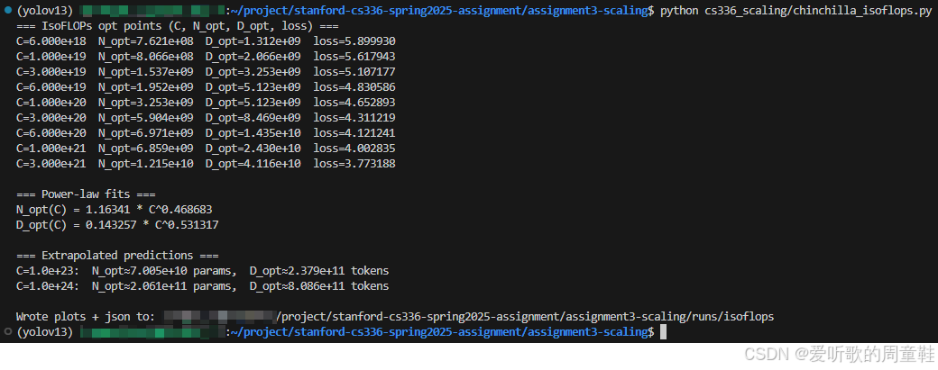
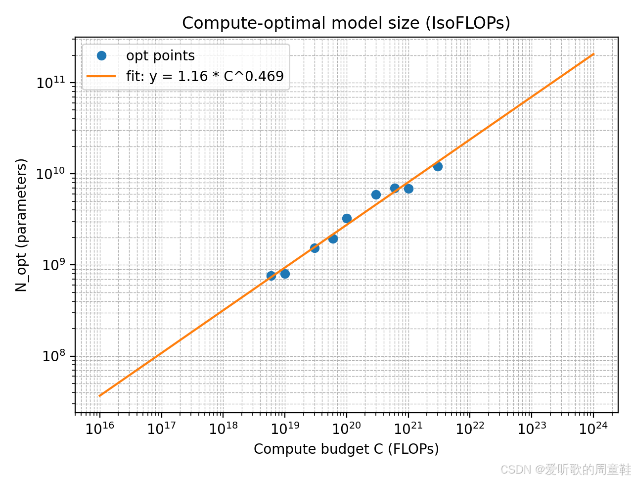
模型规模随计算预算变化的缩放定律图如下所示：

数据集规模随计算预算变化的缩放定律图如下所示：

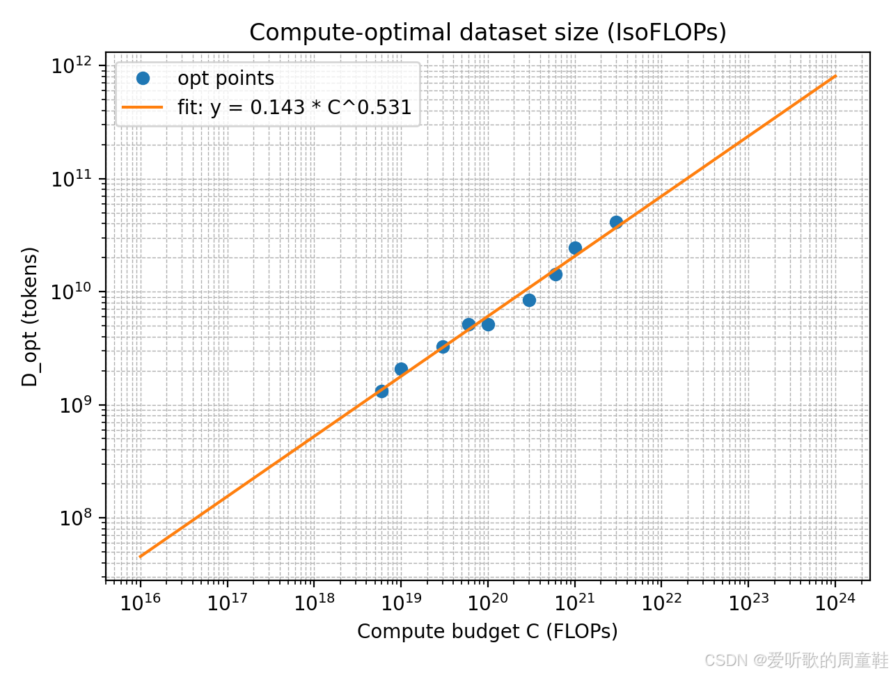
我们使用给定的 IsoFLOPs 曲线数据，在每个计算预算 $C_i$ 下，从不同模型规模的多次训练结果中选择 final loss 最小 的那条 run 作为该预算下的 compute-optimal 点，得到一组最优点 $\{(C_i,N_{\text{opt}}(C_i))\}$。随后利用 Chinchilla 常用近似计算公式

$$C\approx 6ND$$

将每个最优点对应的数据规模恢复为

$$D_{\text{opt}}(C_i)=\frac{C_i}{6N_{\text{opt}}}(C_i)$$

基于这些最优点，我们在 log-log 空间对 $N_{\text{opt}}(C)$ 与 $D_{\text{opt}}(C)$ 分别拟合幂律关系 $y=k{C}^a$，得到：

• Compute-optimal 模型参数规模
  $$N_{\text{opt}}(C)\approx 1.16341\cdot C^{0.46868}$$
• Compute-optimal 数据 token 规模
  $$D_{\text{opt}}(C)\approx 0.14326\cdot C^{0.53132}$$

拟合得到的指数满足 $0.46868+0.53132\approx 1$，与 $C\approx 6ND$ 的乘法约束一致（即模型规模与数据规模在计算预算增长下分摊增长）。对应的最优点在两张 log-log 图中基本沿拟合直线分布，说明该幂律对给定预算范围内的数据具有良好解释力。

按题目要求将幂律外推到更大计算预算，得到：

• 当 $C=10^{23}$ FLOPs：
  • $N_{\text{opt}}\approx 7.01\times 10^{10}$（约 70B 参数）
  • $D_{\text{opt}}\approx 2.38\times 10^{11}$ tokens（约 238B tokens）
• 当 $C=10^{24}$ FLOPs：
  • $N_{\text{opt}}\approx 2.06\times 10^{11}$（约 206B 参数）
  • $D_{\text{opt}}\approx 8.09\times 10^{11}$ tokens（约 809B tokens）

最后我们来简单分析下代码的实现

上面这份脚本的核心目标是：从 data/isoflops_curves.json 中恢复出 compute budget → compute-optimal 模型规模/数据规模 的缩放规律，并对更大预算做外推。

1) 数据读取与统一字段

@dataclass(frozen=True)
class Run:
    parameters: float       # N
    compute_budget: float   # C
    final_loss: float       # L


def load_runs(path: Path) -> List[Run]:
    data = json.loads(path.read_text())
    runs: List[Run] = []
    for r in data:
        runs.append(
            Run(
                parameters=float(r["parameters"]),
                compute_budget=float(r["compute_budget"]),
                final_loss=float(r["final_loss"]),
            )
        )
    return runs

脚本首先读取 isoflops_curves.json，并将每条实验记录解析为包含三项关键字段的结构：

• parameters：模型参数量 $N$
• compute_budget：计算预算 $C$
• final_loss：该实验的最终 loss

这样后续逻辑就可以直接围绕 $(C,N,\text{loss})$ 操作。

2) IsoFLOPs “最优点” 选择策略

def select_opt_points(runs: List[Run]) -> Dict[float, Run]:
    """For each compute budget C, pick the run with the lowest final_loss"""
    best: Dict[float, Run] = {}
    for r in runs:
        C = r.compute_budget
        if C not in best or r.final_loss < best[C].final_loss:
            best[C] = r
    return best

IsoFLOPs 的关键在于：对每个固定计算预算 $C_i$，从多条不同模型规模的 run 中挑选最终 loss 最小的一条，作为该预算下的 compute-optimal 点。代码里就是按 compute_budget 分组维护一个 best[C]，遍历所有 run 时比较 final_loss 并更新最优项。

最终得到点集 $\{(C_i,N_{\text{opt}}(C_i))\}$，这一步相当于 “沿着每条 IsoFLOPs 曲线取最优点”，避免非最优 run 干扰拟合。

3) 由计算预算反推最优数据规模

def main():
    ...

    # Sort by compute budget
    budgets = np.array(sorted(best.keys()), dtype=np.float64)
    n_opt = np.array([best[C].parameters for C in budgets], dtype=np.float64)
    d_opt = budgets / (6.0 * n_opt)    

得到 $N_{\text{opt}}(C_i)$ 后，脚本用 Chinchilla 常用近似 $C\approx 6ND$，直接计算 $D_{\text{opt}}(C_i)=\frac{C_i}{6N_{\text{opt}}(C_i)}$ 从而把每个预算的 “最优模型规模” 同步转换成 “最优数据 token 规模”。

4) 幂律拟合：log-log 线性回归

def fit_power_law(xs: np.ndarray, ys: np.ndarray) -> Tuple[float, float]:
    """
    Fit y = k * x^a via log-log linear regression:
      log(y) = log(k) + a * log(x)
    Returns (k, a).
    """
    if np.any(xs <= 0) or np.any(ys <= 0):
        raise ValueError("x and y must be positive for log-log fit.")
    lx = np.log(xs)
    ly = np.log(ys)
    a, logk = np.polyfit(lx, ly, deg=1)  # slope=a, intercept=logk
    k = float(np.exp(logk))
    return k, float(a)

为了得到缩放律，我们对 $N_{\text{opt}}(C)$ 和 $D_{\text{opt}}(C)$ 分别拟合幂律 $y=k{C}^a$，做法是将其转成线性形式 $\log y=\log k+a\log C$，然后用 np.polyfit(logC, logy, 1) 求出斜率 $a$ 和截距 $\log k$，最后再 $\exp$ 回去得到 $k$。

5) 可视化与外推预测

def predict_power_law(k: float, a: float, x: np.ndarray) -> np.ndarray:
    return k * (x ** a)


def plot_scaling(
    x_points: np.ndarray,
    y_points: np.ndarray,
    k: float,
    a: float,
    out_path: Path,
    title: str,
    y_label: str,
    x_min: float,
    x_max: float
):
    xs = np.logspace(np.log10(x_min), np.log10(x_max), 300)
    ys = predict_power_law(k, a, xs)

    plt.figure()
    plt.loglog(x_points, y_points, marker="o", linestyle="None", label="opt points")
    plt.loglog(xs, ys, linestyle="-", label=f"fit: y = {k:.3g} * C^{a:.3f}")
    plt.xlabel("Compute budget C (FLOPs)")
    plt.ylabel(y_label)
    plt.title(title)
    plt.grid(True, which="both", linestyle="--", linewidth=0.5)
    plt.legend()
    plt.tight_layout()
    plt.savefig(out_path, dpi=200)
    plt.close()


def main():
    ...

    # Predictions required by the problem
    targets = np.array([1e23, 1e24], dtype=np.float64)
    pred_N = predict_power_law(kN, aN, targets)
    pred_D = predict_power_law(kD, aD, targets)

    # Print results
    print("=== IsoFLOPs opt points (C, N_opt, D_opt, loss) ===")
    for C in budgets:
        r = best[C]
        print(f"C={C:.3e}  N_opt={r.parameters:.3e}  D_opt={C/(6*r.parameters):.3e}  loss={r.final_loss:.6f}")

    print("\n=== Power-law fits ===")
    print(f"N_opt(C) = {kN:.6g} * C^{aN:.6f}")
    print(f"D_opt(C) = {kD:.6g} * C^{aD:.6f}")

    print("\n=== Extrapolated predictions ===")
    for C, Np, Dp in zip(targets, pred_N, pred_D):
        print(f"C={C:.1e}:  N_opt≈{Np:.3e} params,  D_opt≈{Dp:.3e} tokens")    

最后我们用 logspace 生成从观测范围延伸到 $10^{24}$ 的 $C$ 网格，并画两张 log-log 图：

• $C\to N_{\text{opt}}$
• $C\to D_{\text{opt}}$

同时用拟合的 $k,a$ 在 $10^{23},10^{24}$ 处直接计算预测值并打印出来。

2. Problem (scaling_laws): 50 points

构建一套 缩放定律（scaling law） 用于在 1e19 FLOPs 的计算预算下，准确预测最优模型规模、对应的超参数配置以及最终训练损失。为此，你需要使用我们提供的 training API 来查询不同实验配置下的最终训练损失（见 §3.1）。在拟合缩放定律的过程中，你最多只能查询 2e19 FLOPs 规模的实验数据，这是 API 强制执行的硬性上限。

Deliverable：请提交一份排版规范的书面报告，其中应完整、清晰地说明：

• 你用于拟合缩放定律的方法与整体思路；
• 你如何利用该缩放定律，在给定 FLOPs 预算下预测最优模型规模；
• 你最终给出的预测结果。

报告中应包含对关键设计决策的解释，并提供足够细节，使他人可以复现你的方法与结果。

关于 batch size 的说明（重要）

在 1e19 FLOPs 的预算下，你报告的超参数配置中，batch size 必须为 128 或 256。这一限制的目的是确保实验具备足够高的 FLOPs 利用率。如果在运行你所报告的配置时出现显存不足（OOM）问题，我们将通过 梯度累积（gradient accumulation） 或 增加数据并行 GPU 数量 的方式来维持你所指定的 batch size。

建议你在报告中重点回答的问题

为了帮助你顺利开始，我们建议你至少思考并在报告中讨论以下问题（你的 write-up 应对每一点给出额外说明，解释你的决策依据）：

• 在固定的 2e18 FLOPs 缩放定律拟合预算下，你是如何决定要查询哪些训练配置的？
• 你是如何拟合缩放定律的？请详细描述你所使用的具体方法或方法组合。特别的，我们建议你参考 [Kaplan+ 2020] 与 [Hoffmann+ 2022] 中采用的建模思路。
• 你的缩放定律对实验数据的拟合效果如何？
• 在 1e19 FLOPs 的预算下，你的缩放定律预测的最优模型规模是多少？对应的预测训练损失是多少？
• 如果你真的要训练一个具有该预测最优参数规模的模型，你会选择哪些超参数？Tips：对于一个给定模型，其 非 embedding 参数数量 可近似估计为 $12n_{\text{layer}}{d}_{\text{model}}^2$

额外提交要求

除书面报告外，你还需要额外提交以下内容：

1. 你预测的 最优模型规模；

2. 你选择的 训练超参数配置（包括 batch size，必须为 128 或 256）；

3. 你预测的 模型训练损失。

上述三项内容请提交至以下 Google 表单：https://forms.gle/sAUSLwCUETew2hYN6

最终评分中，一部分分数将取决于你所预测的最优模型在实际训练中的表现。

Note：由于缺乏官方 API 的访问权限，本次作业无法进行测试。未来官方可能会通过其他方式开放，请关注官方仓库的相关说明与讨论：stanford-cs336/assignment3-scaling#1

下面我们简单过下相关的测试脚本，最后分析下拟合 scaling laws 的方法与整体思路（注意❗所有脚本均未通过充分的测试，后续如果有数据软件包开放我们再来完成本次作业）

作业的核心目标是：在 1e19 FLOPs 的训练预算下，预测 compute-optimal 的模型规模 + 一套可训练的超参数 + 预测的最终训练损失；我们只能通过 training API 查询实验结果，并且用于 “拟合缩放定律” 的查询总 FLOPs 预算有硬上限（超过就会被拒绝）。

本次作业实现的脚本包括 3 类：

A. API 调用与缓存层

目的：统一调用 GET /loss、查询 GET /total_flops_used、拉取 GET /previous_runs，并把已跑过的配置缓存下来。

相关脚本：

• cs336_scaling/api_client.py
  • get_loss(config) -> loss, total_flops_used
  • get_total_flops_used()
  • get_previous_runs()
• cache.py
• query_api.py

B. 实验设计 / 搜索脚本

目的：在 “拟合预算” 内决定要查哪些点（哪些模型规模、哪些学习率/层数/宽度/heads/batch/train_flops），并尽量高效找到规律。

相关脚本：

• cs336_scaling/run_sweep.py：
  • 支持 grid / 分阶段搜索（先粗扫再细化）
  • 每次查询前先看 total_flops_used

C. 缩放定律拟合与预测脚本

目的：把我们查询到的数据拟合成一个可外推的模型，然后在 1e19 FLOPs 下输出：

• 预测最优模型规模（参数量）
• 对应超参数
• 预测训练损失

相关脚本：

• cs336_scaling/scaling_data.py
• cs336_scaling/fit_scaling_law.py
• cs336_scaling/predict_1e19.py

下面我们就来看看这些脚本是如何实现的，该如何运行

2.1 API 调用与缓存层脚本实现

assignment3-scaling/ 下包括：

cs336_scaling/
  api_client.py        # API 调用 + 参数校验 + 错误处理
  cache.py             # 本地缓存（jsonl / sqlite 都行，这里用 jsonl 最轻）
  query_api.py         # 一个小 CLI：单次/批量查询、导出结果
runs/
  api_cache.jsonl      # 自动生成：缓存与日志

首先来看 本地缓存层 cs336_scaling/cache.py 的实现：

import hashlib
import json
from dataclasses import dataclass
from pathlib import Path
from typing import Any, Dict, Optional


def _stable_json(obj: Any) -> str:
    return json.dumps(obj, sort_keys=True, separators=(",", ":"), ensure_ascii=False)


def make_key(endpoint: str, params: Dict[str, Any]) -> str:
    payload = {"endpoint": endpoint, "params": params}
    h = hashlib.sha256(_stable_json(payload).encode("utf-8")).hexdigest()
    return h


@dataclass
class CacheHit:
    key: str
    value: Dict[str, Any]


class JsonlCache:
    """
    Append-only JSONL cache.
    Each line: {"key":..., "endpoint":..., "params":..., "response":...}
    """

    def __init__(self, path: str | Path):
        self.path = Path(path)
        self.path.parent.mkdir(parents=True, exist_ok=True)
        self._index: Dict[str, Dict[str, Any]] = {}
        if self.path.exists():
            self._load()

    def _load(self) -> None:
        with self.path.open("r", encoding="utf-8") as f:
            for line in f:
                line = line.strip()
                if not line:
                    continue
                obj = json.loads(line)
                key = obj.get("key")
                if key:
                    self._index[key] = obj
    
    def get(self, endpoint: str, params: Dict[str, Any]) -> Optional[CacheHit]:
        key = make_key(endpoint, params)
        obj = self._index.get(key)
        if obj is None:
            return None
        return CacheHit(key=key, value=obj["response"])
    
    def put(self, endpoint: str, params: Dict[str, Any], response: Dict[str, Any]) -> str:
        key = make_key(endpoint, params)
        record = {
            "key": key,
            "endpoint": endpoint,
            "params": params,
            "response": response,
        }
        with self.path.open("a", encoding="utf-8") as f:
            f.write(_stable_json(record) + "\n")
        self._index[key] = record
        return key

核心目标是 同一请求（endpoint + 参数）只打一次网络，并将结果写成 append-only 的 json，方便 grep / 画图 / 复现。

接着来看 API 调用层 cs336_scaling/api_client.py 的实现：

from dataclasses import dataclass
from typing import Any, Dict

import requests

from cache import JsonlCache


@dataclass(frozen=True)
class LossQuery:
    d_model: int
    num_layers: int
    num_heads: int
    batch_size: int
    learning_rate: float
    train_flops: int


class ScalingAPIError(RuntimeError):
    pass


class ScalingAPIClient:
    def __init__(
        self,
        api_key: str,
        base_url: str = "http://hyperturing.stanford.edu:8000",
        cache_path: str = "runs/api_cache.jsonl",
        timeout_s: int = 60,
    ):
        self.api_key = api_key
        self.base_url = base_url.rstrip("/")
        self.cache = JsonlCache(cache_path)
        self.timeout_s = timeout_s
    
    # -------------------------
    # Local validation (matches the handout)
    # -------------------------
    def _validate_loss_query(self, q: LossQuery) -> None:
        # Ranges from the handout: d_model[64,1024], layers[2,24], heads[2,16],
        # batch_size[128,256], lr[1e-4,1e-3], train_flops in a fixed set. :contentReference[oaicite:5]{index=5}
        if not (64 <= q.d_model <= 1024):
            raise ValueError(f"d_model out of range: {q.d_model}")
        if not (2 <= q.num_layers <= 24):
            raise ValueError(f"num_layers out of range: {q.num_layers}")
        if not (2 <= q.num_heads <= 16):
            raise ValueError(f"num_heads out of range: {q.num_heads}")
        if not (128 <= q.batch_size <= 256):
            raise ValueError(f"batch_size out of range: {q.batch_size}")
        if not (1e-4 <= q.learning_rate <= 1e-3):
            raise ValueError(f"learning_rate out of range: {q.learning_rate}")

        allowed = {
            int(1e13), int(3e13), int(6e13),
            int(1e14), int(3e14), int(6e14),
            int(1e15), int(3e15), int(6e15),
            int(1e16), int(3e16), int(6e16),
            int(1e17), int(3e17), int(6e17),
            int(1e18),
        }
        if int(q.train_flops) not in allowed:
            raise ValueError(f"train_flops not allowed: {q.train_flops}")

    def _get_json(self, path: str, params: Dict[str, Any]) -> Dict[str, Any]:
        url = f"{self.base_url}/{path.lstrip('/')}"
        r = requests.get(url, params=params, timeout=self.timeout_s)
        # API error examples return {"message": "..."} :contentReference[oaicite:6]{index=6}:contentReference[oaicite:7]{index=7}
        try:
            payload = r.json()
        except Exception as e:
            raise ScalingAPIError(f"Non-JSON response: status={r.status_code}, text={r.text[:200]}") from e

        if r.status_code != 200:
            msg = payload.get("message", payload)
            raise ScalingAPIError(f"API error {r.status_code} @ {url}: {msg}")
        return payload

    # -------------------------
    # Public endpoints
    # -------------------------
    def total_flops_used(self) -> float:
        endpoint = "/total_flops_used"            
        params = {"api_key": self.api_key}
        hit = self.cache.get(endpoint, params)
        if hit:
            return float(hit.value)
        out = self._get_json(endpoint, params)
        # sample shows it returns a number (JSON scalar) :contentReference[oaicite:8]{index=8}
        self.cache.put(endpoint, params, out)
        return float(out)

    def previous_runs(self) -> Dict[str, Any]:
        endpoint = "/previous_runs"
        params = {"api_key": self.api_key}
        hit = self.cache.get(endpoint, params)
        if hit:
            return hit.value
        out = self._get_json(endpoint, params)
        self.cache.put(endpoint, params, out)
        return out

    def loss(self, q: LossQuery, use_cache: bool = True) -> Dict[str, Any]:
        self._validate_loss_query(q)

        endpoint = "/loss"
        params = {
            "d_model": q.d_model,
            "num_layers": q.num_layers,
            "num_heads": q.num_heads,
            "batch_size": q.batch_size,
            "learning_rate": q.learning_rate,
            "train_flops": int(q.train_flops),
            "api_key": self.api_key,            
        }

        if use_cache:
            hit = self.cache.get(endpoint, params)
            if hit:
                return hit.value
        
        out = self._get_json(endpoint, params)
        # example output: {"loss": ..., "total_flops_used": ...} :contentReference[oaicite:9]{index=9}
        self.cache.put(endpoint, params, out)
        return out

上述脚本把 三个端点 都封装了起来，并提供：

• 参数范围的本地校验（避免无意义 404 请求）
• 自动走缓存
• 错误信息更清晰

最后 一个最小 CLI cs336_scaling/query_api.py 的实现如下：

import argparse
import os
from pprint import pprint

from api_client import LossQuery, ScalingAPIClient


def main():
    p = argparse.ArgumentParser()
    p.add_argument("--api-key", default=os.environ.get("CS336_API_KEY", ""))
    p.add_argument("--base-url", default="http://hyperturing.stanford.edu:8000")
    p.add_argument("--cache", default="runs/api_cache.jsonl")

    sub = p.add_subparsers(dest="cmd", required=True)

    sub.add_parser("total_flops_used")
    sub.add_parser("previous_runs")

    q = sub.add_parser("loss")
    q.add_argument("--d-model", type=int, required=True)
    q.add_argument("--num-layers", type=int, required=True)
    q.add_argument("--num-heads", type=int, required=True)
    q.add_argument("--batch-size", type=int, required=True)
    q.add_argument("--learning-rate", type=float, required=True)
    q.add_argument("--train-flops", type=int, required=True)

    args = p.parse_args()
    if not args.api_key:
        raise SystemExit("Missing --api-key or env CS336_API_KEY")

    client = ScalingAPIClient(
        api_key=args.api_key,
        base_url=args.base_url,
        cache_path=args.cache,
    )

    if args.cmd == "total_flops_used":
        print(client.total_flops_used())
        return

    if args.cmd == "previous_runs":
        pprint(client.previous_runs())
        return

    if args.cmd == "loss":
        out = client.loss(
            LossQuery(
                d_model=args.d_model,
                num_layers=args.num_layers,
                num_heads=args.num_heads,
                batch_size=args.batch_size,
                learning_rate=args.learning_rate,
                train_flops=args.train_flops,
            )
        )
        pprint(out)
        return


if __name__ == "__main__":
    main()

该脚本能让我们快速验证：key 是否能用、缓存是否生效以及单条 loss 查询流程是否畅通。

执行指令如下：

# 建议用环境变量放 key（避免出现在 shell history）
export CS336_API_KEY="你的key(SSH公钥字符串，没换行)"

# 1) 先验证 key & 网络
uv run python cs336_scaling/query_api.py total_flops_used

# 2) 看看历史 runs（也会进缓存）
uv run python cs336_scaling/query_api.py previous_runs

# 3) 单条 loss 查询（参数范围见 handout）
uv run python cs336_scaling/query_api.py loss \
  --d-model 1024 --num-layers 24 --num-heads 16 \
  --batch-size 128 --learning-rate 0.001 --train-flops 10000000000000000

连续跑两次相同的 loss 命令时，第二次应直接命中 runs/api_cache.jsonl，不会再发请求。

2.2 实验设计 / 搜索脚本实现

cs336_scaling/run_sweep.py 实现如下：

import argparse
import json
import os
import time
from dataclasses import asdict
from pathlib import Path
from typing import Dict, Iterable, List

from api_client import LossQuery, ScalingAPIClient, ScalingAPIError


# -----------------------------
# Utilities
# -----------------------------
def now_ms() -> int:
    return int(time.time() * 1000)


def jsonl_append(path: Path, obj: Dict) -> None:
    path.parent.mkdir(parents=True, exist_ok=True)
    with path.open("a", encoding="utf-8") as f:
        f.write(json.dumps(obj, ensure_ascii=False) + "\n")


def iter_unique(seq: Iterable[LossQuery]) -> List[LossQuery]:
    seen = set()
    out: List[LossQuery] = []
    for q in seq:
        key = (
            q.d_model,
            q.num_layers,
            q.num_heads,
            q.batch_size,
            float(q.learning_rate),
            int(q.train_flops),
        )
        if key in  seen:
            continue
        seen.add(key)
        out.append(q)
    return out


def estimate_nonemb_params(d_model: int, num_layers: int) -> float:
    # Handout tip: non-embedding params ≈ 12 * n_layer * d_model^2
    return 12.0 * num_layers * (d_model ** 2)


# -----------------------------
# Grid generator (coarse -> refine)
# -----------------------------
def coarse_grid(
    train_flops: List[int],
    batch_sizes: List[int],
    d_models: List[int],
    num_layers: List[int],
    num_heads: List[int],
    learning_rates: List[float],
) -> List[LossQuery]:
    """
    Coarse exploration:
      - fewer shapes
      - a couple lrs
      - multiple compute levels
    """
    qs: List[LossQuery] = []
    for C in train_flops:
        for bs in batch_sizes:
            for d in d_models:
                for nl in num_layers:
                    for nh in num_heads:
                        # require d_model divisible by num_heads (Transformer constraint)
                        if d % nh != 0:
                            continue
                        for lr in learning_rates:
                            qs.append(
                                LossQuery(
                                    d_model=d,
                                    num_layers=nl,
                                    num_heads=nh,
                                    batch_size=bs,
                                    learning_rate=lr,
                                    train_flops=int(C),
                                )
                            )
    return iter_unique(qs)


def refine_grid_around_best(
    best: LossQuery,
    train_flops: List[int],
    batch_sizes: List[int],
    d_model_mults: List[float],
    layer_deltas: List[int],
    head_candidates: List[int],
    lr_mults: List[float],
) -> List[LossQuery]:
    """
    Local refinement around a "best" config (by loss at some compute).
    """
    qs: List[LossQuery] = []
    for C in train_flops:
        for bs in batch_sizes:
            for dm in d_model_mults:
                d = int(round(best.d_model * dm))
                d = max(64, min(1024, d))  # API range :contentReference[oaicite:9]{index=9}
                for dl in layer_deltas:
                    nl = best.num_layers + dl
                    nl = max(2, min(24, nl))  # API range :contentReference[oaicite:10]{index=10}
                    for nh in head_candidates:
                        if d % nh != 0:
                            continue
                        for lm in lr_mults:
                            lr = float(best.learning_rate * lm)
                            # clamp to API range [1e-4, 1e-3] :contentReference[oaicite:11]{index=11}
                            lr = max(1e-4, min(1e-3, lr))
                            qs.append(
                                LossQuery(
                                    d_model=d,
                                    num_layers=nl,
                                    num_heads=nh,
                                    batch_size=bs,
                                    learning_rate=lr,
                                    train_flops=int(C),
                                )
                            )
    return iter_unique(qs)


# -----------------------------
# Budget-aware runner
# -----------------------------
def would_consume_budget(client: ScalingAPIClient, q: LossQuery) -> bool:
    """
    If cache already has this exact request, then it's free (no extra FLOPs):contentReference[oaicite:12]{index=12}.
    We check client.cache directly via the endpoint+params mapping used in api_client.py.
    """
    endpoint = "/loss"
    params = {
        "d_model": q.d_model,
        "num_layers": q.num_layers,
        "num_heads": q.num_heads,
        "batch_size": q.batch_size,
        "learning_rate": q.learning_rate,
        "train_flops": int(q.train_flops),
        "api_key": client.api_key,        
    }
    hit = client.cache.get(endpoint, params)
    return hit is None


def run_queries(
    client: ScalingAPIClient,
    queries: List[LossQuery],
    max_fit_budget_flops: float = 2e18,
    results_path: Path = Path("runs/sweep_results.jsonl"),
    dry_run: bool = False,
    sleep_s: float = 0.0,
) -> None:
    """
    Executes queries until (estimated) budget would exceed max_fit_budget_flops.
    Notes:
      - total_flops_used is returned by API and can be fetched anytime:contentReference[oaicite:13]{index=13}.
      - If we exceed the 2e18 scaling-law budget, API will refuse future requests:contentReference[oaicite:14]{index=14},
        so we stop conservatively.
    """
    # starting point from API
    try:
        used0 = float(client.total_flops_used())
    except ScalingAPIError:
        # If key has never queried, the endpoint may 422; but in that case used0=0 is safe.
        used0 = 0.0

    planned_new = 0.0
    n_new = 0
    n_cached = 0

    # Pre-pass: compute how many are cached & estimated extra FLOPs
    for q in queries:
        if would_consume_budget(client, q):
            planned_new += float(q.train_flops)
            n_new += 1
        else:
            n_cached += 1

    print("=== Sweep plan ===")
    print(f"queries_total: {len(queries)}")
    print(f"cached_free:   {n_cached}")
    print(f"new_queries:   {n_new}")
    print(f"api_used_now:  {used0:.3e} FLOPs")
    print(f"est_new_cost:  {planned_new:.3e} FLOPs")
    print(f"est_total:     {(used0 + planned_new):.3e} FLOPs")
    print(f"budget_limit:  {max_fit_budget_flops:.3e} FLOPs")

    if dry_run:
        print("\n[dry-run] not executing API calls.")
        return

    # Execute with conservative budget guard
    used = used0
    for i, q in enumerate(queries):
        is_new = would_consume_budget(client, q)
        est_after = used + (float(q.train_flops) if is_new else 0.0)

        if est_after > max_fit_budget_flops:
            print(
                f"[STOP] Budget guard: would exceed limit if running next query. "
                f"used={used:.3e}, next_cost={(q.train_flops if is_new else 0):.3e}, "
                f"limit={max_fit_budget_flops:.3e}"
            )
            return

        rec = {
            "ts_ms": now_ms(),
            "index": i,
            "query": asdict(q),
            "nonemb_params_est": estimate_nonemb_params(q.d_model, q.num_layers),
            "was_cached": (not is_new),
        }

        try:
            out = client.loss(q, use_cache=True)
            rec["response"] = out
            # Use authoritative used FLOPs if API returns it in /loss response:contentReference[oaicite:15]{index=15}
            if isinstance(out, dict) and "total_flops_used" in out:
                used = float(out["total_flops_used"])
            else:
                # fallback estimate
                used = est_after
            rec["api_used_after"] = used
            rec["status"] = "ok"
            print(
                f"[{i+1}/{len(queries)}] ok "
                f"C={q.train_flops:.1e} d={q.d_model} L={q.num_layers} H={q.num_heads} "
                f"bs={q.batch_size} lr={q.learning_rate:g} "
                f"loss={out.get('loss', None)} used={used:.3e}"
            )
        except Exception as e:
            rec["status"] = "error"
            rec["error"] = repr(e)
            print(f"[{i+1}/{len(queries)}] error: {e!r}")

        jsonl_append(results_path, rec)

        if sleep_s > 0:
            time.sleep(sleep_s)


# -----------------------------
# CLI
# -----------------------------
def main():
    p = argparse.ArgumentParser()
    p.add_argument("--api-key", default=os.environ.get("CS336_API_KEY", ""))
    p.add_argument("--base-url", default="http://hyperturing.stanford.edu:8000")
    p.add_argument("--cache", default="runs/api_cache.jsonl")
    p.add_argument("--out", default="runs/sweep_results.jsonl")
    p.add_argument("--budget", type=float, default=2e18, help="scaling-law fit budget cap (FLOPs)")
    p.add_argument("--dry-run", action="store_true")
    p.add_argument("--sleep", type=float, default=0.0)

    sub = p.add_subparsers(dest="mode", required=True)

    # coarse mode
    c = sub.add_parser("coarse")
    c.add_argument("--train-flops", nargs="+", type=float, default=[1e13, 1e14, 1e15, 1e16, 1e17, 1e18])
    c.add_argument("--batch-sizes", nargs="+", type=int, default=[128])
    c.add_argument("--d-models", nargs="+", type=int, default=[128, 256, 512, 768, 1024])
    c.add_argument("--num-layers", nargs="+", type=int, default=[2, 4, 8, 12, 16, 24])
    c.add_argument("--num-heads", nargs="+", type=int, default=[2, 4, 8, 16])
    c.add_argument("--learning-rates", nargs="+", type=float, default=[1e-4, 3e-4, 1e-3])

    # refine mode: requires a seed config
    r = sub.add_parser("refine")
    r.add_argument("--seed-d-model", type=int, required=True)
    r.add_argument("--seed-num-layers", type=int, required=True)
    r.add_argument("--seed-num-heads", type=int, required=True)
    r.add_argument("--seed-batch-size", type=int, required=True)
    r.add_argument("--seed-learning-rate", type=float, required=True)
    r.add_argument("--train-flops", nargs="+", type=float, default=[1e16, 3e16, 1e17, 3e17, 1e18])
    r.add_argument("--batch-sizes", nargs="+", type=int, default=[128, 256])
    r.add_argument("--d-model-mults", nargs="+", type=float, default=[0.75, 1.0, 1.25])
    r.add_argument("--layer-deltas", nargs="+", type=int, default=[-2, 0, 2])
    r.add_argument("--head-candidates", nargs="+", type=int, default=[2, 4, 8, 16])
    r.add_argument("--lr-mults", nargs="+", type=float, default=[0.5, 1.0, 2.0])

    args = p.parse_args()
    if not args.api_key:
        raise SystemExit("Missing --api-key or env CS336_API_KEY")

    client = ScalingAPIClient(
        api_key=args.api_key,
        base_url=args.base_url,
        cache_path=args.cache,
    )

    out_path = Path(args.out)

    if args.mode == "coarse":
        queries = coarse_grid(
            train_flops=[int(x) for x in args.train_flops],
            batch_sizes=args.batch_sizes,
            d_models=args.d_models,
            num_layers=args.num_layers,
            num_heads=args.num_heads,
            learning_rates=args.learning_rates,
        )

    else:
        seed = LossQuery(
            d_model=args.seed_d_model,
            num_layers=args.seed_num_layers,
            num_heads=args.seed_num_heads,
            batch_size=args.seed_batch_size,
            learning_rate=args.seed_learning_rate,
            train_flops=int(1e13),  # placeholder; replaced by --train-flops below
        )
        queries = refine_grid_around_best(
            best=seed,
            train_flops=[int(x) for x in args.train_flops],
            batch_sizes=args.batch_sizes,
            d_model_mults=args.d_model_mults,
            layer_deltas=args.layer_deltas,
            head_candidates=args.head_candidates,
            lr_mults=args.lr_mults,
        )

    run_queries(
        client=client,
        queries=queries,
        max_fit_budget_flops=float(args.budget),
        results_path=out_path,
        dry_run=bool(args.dry_run),
        sleep_s=float(args.sleep),
    )


if __name__ == "__main__":
    main()

上面这个脚本的目标是生成一批 LossQuery，在每次真正 query 前，先检查：

1. 这个配置是否已在本地 cache / API 历史中出现（出现则不计预算）

2. 若是新配置，估算新增消耗是否会让总 FLOPs 超过 2e18（超了就停）

执行流程如下：

0) 先 dry-run 看预算会不会爆

我们的预算上限是 2e18 FLOPs，超过会被拒绝后续请求，所以先 dry-run 让脚本算一遍预计消耗最稳

export CS336_API_KEY="你的key"

uv run python cs336_scaling/run_sweep.py --dry-run coarse \
  --train-flops 1e13 1e14 1e15 1e16 1e17 1e18 \
  --batch-sizes 128 \
  --d-models 128 256 512 1024 \
  --num-layers 2 4 8 16 24 \
  --num-heads 2 4 8 16 \
  --learning-rates 1e-4 3e-4 1e-3

脚本会输出：总 query 数、cache 命中数、新 query 数、预计新增 FLOPs、预计总 FLOPs。

1) 正式跑 coarse sweep（会写 jsonl 结果）

uv run python cs336_scaling/run_sweep.py coarse \
  --train-flops 1e13 1e14 1e15 1e16 1e17 1e18 \
  --batch-sizes 128 \
  --d-models 128 256 512 1024 \
  --num-layers 2 4 8 16 24 \
  --num-heads 2 4 8 16 \
  --learning-rates 1e-4 3e-4 1e-3

输出会放在：

• runs/api_cache.jsonl：缓存
• runs/sweep_results.jsonl：本次 sweep 的逐条记录：query、loss、used flops、是否 cache 命中等

2) 选一个 coarse 最优点作为 seed，然后 refin

uv run python cs336_scaling/run_sweep.py refine \
  --seed-d-model 512 --seed-num-layers 16 --seed-num-heads 8 \
  --seed-batch-size 128 --seed-learning-rate 0.0003 \
  --train-flops 1e16 3e16 1e17 3e17 1e18

我们再从 runs/sweep_results.jsonl 里找某个 compute（比如 train_flops=1e18）下 loss 最低的配置，当作 seed

2.3 缩放定律拟合与预测脚本实现

整体拟合和外推设计思路如下：

1. 从 sweep_results.jsonl 汇总数据：每条记录里有 query（d_model/layers/heads/batch/lr/train_flops） 和 response.loss

2. 把结构超参映射到模型规模 N：用作业建议的 tip 近似：$N_{\text{non-emb}}\approx 12n_{\text{layer}}{d}_{\text{model}}^2$

3. IsoFLOPs-stype 的 “每个 compute 取最优点”：对每个 train_flops = C，选 loss 最小的配置作为 $((C,N_{\text{opt}}(C),L_{\text{opt}}(C)))$

4. 在 log-log 空间拟合两条幂律：

• 最优模型规模：$N_{\text{opt}}(C)=k_N,C^{a_N}$
• 最优 loss：$L_{\text{opt}}(C)=L_{\infty }+k_L{C}^{-a_L}$（带一个不可达下界 $L_{\infty }$，比纯幂律更稳）

5. 外推到 1e19：得到 $N_{\text{opt}}(1e19)$ 和 $L_{\text{opt}}(1e19)$

6. 给出 1e19 的 “可提交超参”：在允许范围内找一个结构 $(d_{\text{model}},n_{\text{layer}},n_{\text{head}})$ 使得估算参数量最接近 $N_{\text{opt}}(1e19)$，batch 取 256（或 128），learning rate 取在最大 compute（1e18）附近表现最好的 lr（也可以按 lr 随 compute 的经验趋势做轻微外推）。

首先 数据汇总工具 cs336_scaling/scaling_data.py 的实现如下：

import json
from dataclasses import dataclass
from pathlib import Path
from typing import Dict, Iterable, List, Optional, Tuple


@dataclass(frozen=True)
class RunRow:
    d_model: int
    num_layers: int
    num_heads: int
    batch_size: int
    learning_rate: float
    train_flops: int
    loss: float


def approx_nonemb_params(d_model: int, num_layers: int) -> float:
    # Handout tip: non-embedding params ≈ 12 * n_layer * d_model^2
    return 12.0 * num_layers * (d_model ** 2)


def load_sweep_jsonl(path: str | Path) -> List[RunRow]:
    path = Path(path)
    rows: List[RunRow] = []
    if not path.exists():
        raise FileNotFoundError(path)

    with path.open("r", encoding="utf-8") as f:
        for line in f:
            line = line.strip()
            if not line:
                continue
            obj = json.loads(line)
            if obj.get("status") != "ok":
                continue
            q = obj.get("query", {})
            resp = obj.get("response", {})
            if "loss" not in resp:
                continue
            rows.append(
                RunRow(
                    d_model=int(q["d_model"]),
                    num_layers=int(q["num_layers"]),
                    num_heads=int(q["num_heads"]),
                    batch_size=int(q["batch_size"]),
                    learning_rate=float(q["learning_rate"]),
                    train_flops=int(q["train_flops"]),
                    loss=float(resp["loss"]),
                )
            )


def group_best_by_compute(rows: Iterable[RunRow]) -> Dict[int, RunRow]:
    best: Dict[int, RunRow] = {}
    for r in rows:
        C = r.train_flops
        if (C not in best) or (r.loss < best[C].loss):
            best[C] = r
    return best

拟合脚本 cs336_scaling/fit_scaling_laws.py 的实现如下：

import argparse
import csv
import json
from pathlib import Path
from typing import Dict, Tuple

import numpy as np
import matplotlib.pyplot as plt

from scaling_data import approx_nonemb_params, group_best_by_compute, load_sweep_jsonl


def fit_powerlaw(x: np.ndarray, y: np.ndarray) -> Tuple[float, float]:
    """
    Fit y = k * x^a using log-log linear regression.
    Returns (k, a).
    """
    lx = np.log(x)
    ly = np.log(y)
    a, logk = np.polyfit(lx, ly, 1)
    return float(np.exp(logk)), float(a)


def fit_loss_with_floor(C: np.ndarray, L: np.ndarray) -> Dict[str, float]:
    """
    Fit L(C) = L_inf + k * C^{-a}
    via a simple grid search over L_inf and log-log fit on (L - L_inf).
    This is robust and dependency-free.
    """
    # L_inf must be below min(L)
    Lmin = float(np.min(L))
    # a conservative grid: from Lmin-2.0 down to Lmin-0.01
    # (you can widen if needed)
    candidates = np.linspace(Lmin - 2.0, Lmin - 0.01, 200)

    best = {"L_inf": None, "k": None, "a": None, "mse": float("inf")}
    for Linf in candidates:
        y = L - Linf
        if np.any(y <= 0):
            continue
        k, a = fit_powerlaw(C, y)          # y = k * C^a, but we need y = k * C^{-aL}
        # In our parameterization: y = k * C^{-aL} => log y = log k - aL log C
        # So slope returned is a = -aL
        aL = -a
        pred = Linf + k * (C ** (-aL))
        mse = float(np.mean((pred - L) ** 2))
        if mse < best["mse"]:
            best = {"L_inf": float(Linf), "k": float(k), "a": float(aL), "mse": mse}

    if best["L_inf"] is None:
        raise RuntimeError("Failed to fit L(C)=L_inf+k*C^{-a}: no valid Linf candidate.")
    return best


def plot_loglog_points_and_fit(x, y, fit_fn, out_path: Path, title: str, ylab: str):
    xs = np.logspace(np.log10(min(x)), np.log10(max(x)), 300)
    ys = fit_fn(xs)
    plt.figure()
    plt.loglog(x, y, marker="o", linestyle="None", label="best points")
    plt.loglog(xs, ys, linestyle="-", label="fit")
    plt.xlabel("Compute budget C (FLOPs)")
    plt.ylabel(ylab)
    plt.title(title)
    plt.grid(True, which="both", linestyle="--", linewidth=0.5)
    plt.legend()
    plt.tight_layout()
    plt.savefig(out_path, dpi=200)
    plt.close()



def main():
    ap = argparse.ArgumentParser()
    ap.add_argument("--sweep", type=Path, default=Path("runs/sweep_results.jsonl"))
    ap.add_argument("--outdir", type=Path, default=Path("runs/scaling_fit"))
    ap.add_argument("--make-plots", action="store_true")
    args = ap.parse_args()

    rows = load_sweep_jsonl(args.sweep)
    best = group_best_by_compute(rows)

    # Sort by compute
    Cs = np.array(sorted(best.keys()), dtype=np.float64)
    Ns = np.array([approx_nonemb_params(best[int(C)].d_model, best[int(C)].num_layers) for C in Cs], dtype=np.float64)
    Ls = np.array([best[int(C)].loss for C in Cs], dtype=np.float64)

    # Fit N_opt(C) = kN * C^aN
    kN, aN = fit_powerlaw(Cs, Ns)

    # Fit L_opt(C) = L_inf + kL * C^{-aL}
    loss_fit = fit_loss_with_floor(Cs, Ls)

    args.outdir.mkdir(parents=True, exist_ok=True)

    # Save points (for writeup tables / plots)
    csv_path = args.outdir / "scaling_fit_points.csv"
    with csv_path.open("w", newline="", encoding="utf-8") as f:
        w = csv.writer(f)
        w.writerow(["train_flops", "loss_best", "d_model", "num_layers", "num_heads", "batch_size", "learning_rate", "n_nonemb_params_est"])
        for C in Cs:
            r = best[int(C)]
            w.writerow([
                int(C), r.loss, r.d_model, r.num_layers, r.num_heads, r.batch_size, r.learning_rate,
                approx_nonemb_params(r.d_model, r.num_layers),
            ])

    # Save fit params
    out = {
        "best_points": [
            {
                "train_flops": int(C),
                "loss": float(best[int(C)].loss),
                "d_model": int(best[int(C)].d_model),
                "num_layers": int(best[int(C)].num_layers),
                "num_heads": int(best[int(C)].num_heads),
                "batch_size": int(best[int(C)].batch_size),
                "learning_rate": float(best[int(C)].learning_rate),
                "n_nonemb_params_est": float(approx_nonemb_params(best[int(C)].d_model, best[int(C)].num_layers)),
            }
            for C in Cs
        ],
        "fit": {
            "n_opt": {"k": kN, "a": aN, "form": "N_opt(C)=k*C^a"},
            "l_opt": {
                "L_inf": loss_fit["L_inf"],
                "k": loss_fit["k"],
                "a": loss_fit["a"],
                "mse": loss_fit["mse"],
                "form": "L_opt(C)=L_inf + k*C^{-a}",
            },
        },
    }
    (args.outdir / "scaling_fit.json").write_text(json.dumps(out, indent=2))

    print("=== Fit results ===")
    print(f"N_opt(C) = {kN:.6g} * C^{aN:.6f}")
    print(f"L_opt(C) = {loss_fit['L_inf']:.6f} + {loss_fit['k']:.6g} * C^(-{loss_fit['a']:.6f})")
    print(f"Saved: {args.outdir/'scaling_fit.json'}")
    print(f"Saved: {csv_path}")

    if args.make_plots:
        plot_loglog_points_and_fit(
            Cs, Ns,
            lambda x: kN * (x ** aN),
            args.outdir / "nopt_vs_c.png",
            title="Compute-optimal model size (from best-per-C points)",
            ylab="N_nonemb_params_est",
        )
        # For loss, loglog doesn't work with floor directly; plot (L-L_inf) for loglog visualization
        Linf = loss_fit["L_inf"]
        y = Ls - Linf
        plot_loglog_points_and_fit(
            Cs, y,
            lambda x: loss_fit["k"] * (x ** (-loss_fit["a"])),
            args.outdir / "lopt_minus_linf_vs_c.png",
            title="Compute-optimal loss gap (L - L_inf)",
            ylab="L_opt - L_inf",
        )
        print("Saved plots to outdir.")


if __name__ == "__main__":
    main()

执行后的输出包括：

• runs/scaling_fit.json：拟合参数 + 每个 compute 的最优点
• runs/scaling_fit_points.csv：方便后续绘图
• 两张图

预测脚本 cs336_scaling/predict_1e19.py 的实现如下：

import argparse
import json
from dataclasses import asdict
from pathlib import Path
from typing import Dict, Tuple

import numpy as np

from api_client import LossQuery
from scaling_data import approx_nonemb_params


ALLOWED_D_MODEL = [64, 96, 128, 160, 192, 256, 320, 384, 512, 640, 768, 896, 1024]
ALLOWED_LAYERS = list(range(2, 25))  # 2..24
ALLOWED_HEADS = [2, 4, 8, 16]
ALLOWED_BATCH = [128, 256]


def find_closest_arch(target_N: float) -> Tuple[Dict, float]:
    """
    brute-force search over allowed ranges to find (d_model, num_layers, num_heads)
    that yields N_est closest to target_N, with d_model % num_heads == 0.
    """
    best = None
    best_err = float("inf")
    best_N = None

    for d in ALLOWED_D_MODEL:
        for nl in ALLOWED_LAYERS:
            for nh in ALLOWED_HEADS:
                if d % nh != 0:
                    continue
                N = approx_nonemb_params(d, nl)
                err = abs(N - target_N) / target_N
                if err < best_err:
                    best_err = err
                    best = {"d_model": d, "num_layers": nl, "num_heads": nh}
                    best_N = N
    return best, float(best_N)


def main():
    ap = argparse.ArgumentParser()
    ap.add_argument("--fit", type=Path, default=Path("runs/scaling_fit/scaling_fit.json"))
    ap.add_argument("--budget", type=float, default=1e19)
    ap.add_argument("--batch", type=int, choices=ALLOWED_BATCH, default=256)
    ap.add_argument("--lr", type=float, default=None, help="override learning rate; if None, use lr from best point at max C")
    args = ap.parse_args()

    data = json.loads(args.fit.read_text())
    nfit = data["fit"]["n_opt"]
    lfit = data["fit"]["l_opt"]

    C = float(args.budget)

    # Predictions
    N_pred = float(nfit["k"]) * (C ** float(nfit["a"]))
    L_pred = float(lfit["L_inf"]) + float(lfit["k"]) * (C ** (-float(lfit["a"])))

    # pick lr from the best point at maximum observed C (usually 1e18) unless overridden
    best_points = data["best_points"]
    maxC_point = max(best_points, key=lambda x: x["train_flops"])
    lr = float(args.lr) if args.lr is not None else float(maxC_point["learning_rate"])

    arch, N_arch = find_closest_arch(N_pred)

    suggested = LossQuery(
        d_model=int(arch["d_model"]),
        num_layers=int(arch["num_layers"]),
        num_heads=int(arch["num_heads"]),
        batch_size=int(args.batch),
        learning_rate=float(lr),
        train_flops=int(1e18),  # API only supports up to 1e18; 1e19 is for your final report prediction
    )

    print("=== Scaling-law prediction at 1e19 FLOPs ===")
    print(f"Predicted N_opt (non-emb est) : {N_pred:.3e}")
    print(f"Predicted L_opt               : {L_pred:.6f}")
    print()
    print("=== Closest feasible architecture (API domain) ===")
    print(f"arch = {arch}, N_est={N_arch:.3e}, rel_err={abs(N_arch-N_pred)/N_pred:.3%}")
    print()
    print("=== Suggested training hyperparams (submit) ===")
    print(f"batch_size must be 128 or 256 (you chose {args.batch}).")  # handout requirement:contentReference[oaicite:6]{index=6}
    print(f"learning_rate = {lr:g}  (default from best @ max observed compute)")
    print()
    print("NOTE: API train_flops max is 1e18; 1e19 values are extrapolated for the report/submission.")
    print("Suggested config (for Google form):")
    print(json.dumps({
        "model_size_nonemb_params_est": N_arch,   # what you'll report as "model size"
        "arch": arch,
        "batch_size": args.batch,
        "learning_rate": lr,
        "predicted_loss_at_1e19": L_pred,
    }, indent=2))


if __name__ == "__main__":
    main()

该脚本会读 scaling_fit.json 并计算 $N_{\text{opt}}(1e19)$、$L_{\text{opt}}(1e19)$，然后在允许范围内搜索一个 “最接近目标参数量” 的结构超参（d_model/layers/heads），并给出 batch、lr（默认取在最大 compute 最优点的 lr）。

运行指令如下：

# 1) 拟合（可选加 --make-plots）
uv run python cs336_scaling/fit_scaling_laws.py \
  --sweep runs/sweep_results.jsonl \
  --outdir runs/scaling_fit \
  --make-plots

# 2) 外推到 1e19，并输出最终“可提交”三元组
uv run python cs336_scaling/predict_1e19.py \
  --fit runs/scaling_fit/scaling_fit.json \
  --budget 1e19 \
  --batch 256

2.4 整体设计思路分析

在本次作业中，我们需要利用课程提供的 training API 对模型规模、训练计算量与训练损失之间的经验缩放规律（scaling laws）进行建模与分析。目标是在 $10^{19}$ FLOPs 的训练预算下，预测 compute-optimal 的模型规模、对应的训练超参数配置以及最终训练损失。

由于在完成本次作业时博主无法获得官方 API 的访问权限，因此这里我们重点完成 实验设计、建模方法与缩放定律拟合思路的完整阐述；所有依赖真实 API 查询才能得到的数值结果，均在文中以【占位】形式标注，如果后续能访问相应 API 我们再来补齐。

1. 问题背景与约束条件

training API 将完整的训练过程抽象为一个黑盒接口，用户可以通过指定模型结构、优化器超参数以及训练计算预算 $C=\text{train\_flops}$ 查询对应的最终损失。

该问题具有以下关键约束：

• 用于拟合 scaling laws 的 API 查询总计算预算上限为 $2\times 10^{18}$ FLOPs，超过该限制将导致后续请求被拒绝；
• 可选的 train_flops 仅限于给定的离散集合，最大为 $10^{18}$ FLOPs；
• 作业要求预测的目标计算预算为 $10^{19}$ FLOPs，因此所有结论均基于对低于 $10^{18}$ FLOPs 区间的 外推（extrapolation）；
• 最终提交的训练配置中，batch size 必须为 128 或 256。

这些约束共同决定了实验必须在严格的预算控制与合理的建模假设下进行。

2. 实验 pipeline 整体设计

围绕上述约束，我们设计并实现了一套模块化的实验 pipeline，整体流程如下：

1. API 调用与本地缓存：所有 API 查询均通过统一封装的接口完成，并使用本地缓存避免重复消耗计算预算；

2. 预算感知的实验扫描（sweep）：在全局 FLOPs 预算限制下，对不同计算预算和模型结构进行分阶段探索；

3. 缩放定律拟合：从实验结果中构造 compute-optimal 点，并拟合模型规模与损失的缩放规律；

4. 外推与最终预测：将拟合得到的 scaling laws 外推到 $10^{19}$ FLOPs，生成最终可提交的预测结果。

3. 模型规模的估计方法

由于 training API 并未直接提供模型的参数总量，而是通过结构超参数（d_model、num_layers、num_heads）简洁描述模型规模，因此需要一次近似映射关系。

在本实验中，我们采用作业提示中建议的近似公式，将非 embedding 参数量估计为：

$$N\approx 12\cdot n_{\text{layer}}\cdot d_{\text{model}}^2$$

4. Compute-Optimal 点的构造方法

在每一个固定的训练计算预算 $C_i$ 下，API 允许查询多组不同结构与超参数配置。为了构造缩放定律，我们采用 IsoFLOPs 风格 的策略，在每个 $C_i$ 上选取训练损失最小的配置作为该预算下的最优点：

$${\theta }^{\ast }(C_i)=\underset{\theta :\text{train\_flops}=C_i}{\mathrm{argmin}}L(\theta )$$

从而得到一组离散的 compute-optimal 点：

$$\{(C_i,N^{\ast }(C_i),L^{\ast }(C_i)){\}}_{i=1}^m$$

5. Scaling Laws 的建模形式

基于上述 compute-optimal 点，我们分别对模型规模与训练损失拟合缩放定律。

5.1 模型规模的缩放规律

我们假设 compute-optimal 模型规模随计算预算呈幂律增长：

$$N^{\ast }(C)=k_N\cdot C^{a_N}$$

在对数空间中，该关系为线性形式，因此可以通过 log-log 线性回归稳定地估计参数 $k_N$ 与 $a_N$

5.2 训练损失的缩放规律

考虑到训练损失在大计算量下趋于饱和，我们采用带有下界项的幂律模型：

$$L^{\ast }(C)=L_{\infty }+k_L\cdot C^{-a_L}$$

其中 $L_{\infty }$ 表示不可进一步降低的损失下界。实际拟合时，对 $L_{\infty }$ 进行网格搜索，在保证 $L-L_{\infty }>0$ 的前提下，对 $\log (L-L_{\infty })$ 与 $\log C$ 进行线性回归，从而得到稳定的参数估计。

6. 外推到 $10^{19}$ FLOPs 的预测方法

一旦完成缩放定律的拟合，即可将其外推至目标计算预算：

$${\hat{N}}^{\ast }(10^{19})=k_N\cdot (10^{19}{)}^{a_N},{\hat{L}}^{\ast }(10^{19})=L_{\infty }+k_L\cdot (10^{19}{)}^{-a_L}$$

由于 API 对模型结构的取值范围有限，我们还需要将预测得到的最优模型规模 ${\hat{N}}^{\ast }$ 映射为一个 可实现的离散结构。具体做法是，在满足以下约束的结构空间中搜索与 ${\hat{N}}^{\ast }$ 最接近的配置：

• $d_{\text{model}}\mathrm{mod}{n}_{\text{head}}=0$；
• $64\le d_{\text{model}}\le 1024$；
• $2\le n_{\text{layer}}\le 24$。

7. 有限预算下的实验设计策略

在 $2\times 10^{18}$ FLOPs 的总预算限制下，我们采用 两阶段实验策略：

第一阶段 (Coarse sweep)

在多个计算预算级别上，选取少量代表性的模型规模、层数和学习率，快速建立训练损失随计算量变化的整体趋势，并定位潜在的优良结构趋于。

第二阶段（Refine sweep）

围绕高计算预算下表现最优的结构，进行小范围的局部扰动（如轻微调整模型宽度、层数与学习率），以更少的额外计算代价提升 compute-optimal 点的质量。

通过在执行前进行预算估算，并结合缓存机制复用已查询结果，可以确保整个过程始终不超过 API 的预算限制。

具体来说，整个查询策略与预算分配方式如下：

在 coarse 阶段，我们采用先 “覆盖后加密” 的原则：对每个离散的 train_flops 挡位，至少保证存在若干（例如 5-10 个）结构候选点，使得后续在该 compute 上能够可靠地选出最低 loss 的最优点。与此同时，我们显式控制扫描维度的数量：优先扫描对模型容量影响最大的结构维度（d_model 与 num_layers），并仅使用少量学习率候选（例如 2-3 个数量级内的代表值），从而在预算内获得足够的跨尺度信息。对于 num_heads，我们主要将其作为满足结构约束（$d_{\text{model}}\mathrm{mod}{n}_{\text{head}}=0$）的离散选项，而不将其作为 coarse 阶段的主要连续搜索维度。

在 refine 阶段，我们以 coarse 阶段在高 compute 挡位上的最优点作为 seed，并围绕该 seed 作为局部网格扰动，例如对 d_model 做 ±25% 的比例变化、对 num_layers 做 ±2 的增量变化、对 learning rate 做 x0.5/x1/x2 的缩放，这样做的核心原因是：缩放定律拟合最终只依赖每个 compute 的 “最优点边界”，因此把额外预算投入到 “提升最优点质量” 比盲目扩大搜索空间更有效。实现层面，我们在每次执行批量查询前通过脚本统计 “缓存命中 vs 新查询数”，并用新增查询的 train_flops 累加估算额外成本；一旦预计下一条查询会使累计消耗超过 $2\times 10^{18}$ 则提前停止，从而保证不会触发 API 的拒绝机制。

8. 实验结果（待补齐）

运行拟合脚本后，将得到以下结果：

• 每个计算预算 $C_i$ 下的 compute-optimal 配置与对应损失
• 模型规模缩放定律的拟合参数：$N^{\ast }(C)=\underline{}\cdot C^{\underline{}}$
• 训练损失缩放定律的拟合参数：$L^{\ast }(C)=\underline{}+\underline{}\cdot C^{-\underline{}}$
• 对应的可视化图表

9. 在 $10^{19}$ FLOPs 下的最终预测结果（待补齐）

运行预测脚本后，将得到以下结果：

• 预测的 compute-optimal 模型规模：${\hat{N}}^{\ast }(10^{19})=\underline{}$
• 最接近的可行模型结构：$d_{\text{model}}=\underline{},n_{\text{layer}}=\underline{},n_{\text{head}}=\underline{}$
• 训练超参数：$\text{batch\_size}=\underline{},\text{learning\_rate}=\underline{}$
• 预测训练损失：${\hat{L}}^{\ast }(10^{19})=\underline{}$

上述结果即为本次作业最终需要提交的内容。

10. 结果讨论（拟合效果评估、外推不确定性与最终超参选择原则）

在拟合效果评估方面，我们同时采用数值指标与可视化图来判断缩放定律是否可信。数值上，我们报告拟合曲线对 best-per-compute 点的均方差（MSE）/ 决定系数（R^2），并重点观察高 compute 区域的误差，因为该区域对外推到 $10^{19}$ FLOPs 的影响最大。可视化上，我们在 log-log 坐标系绘制 $N^{\ast }(C)$ 与 $(L^{\ast }(C)-L_{\infty })$ 的散点与拟合直线，并进一步检查残差随 compute 是否存在系统性偏差，以识别 “幂律假设在某段尺度失效” 的风险。

由于 API 可查询的最大 train_flops 为 $10^{18}$，本作业在 $10^{19}$ FLOPs 下的预测属于尺度外推，其不确定性主要来自三个方面：第一，幂律拟合本身在观测范围外可能偏离真实曲线；第二，compute-optimal 点是通过有限网格搜索近似得到，仍可能与真实最优存在差距；第三，预测得到的最优参数规模 ${\hat{N}}^{\ast }(10^{19})$ 需要映射到离散结构空间（整数 layers、离散 heads、有限 d_model），因此会引入额外的“结构量化误差”。因此我们在报告中需要明确指出：最终的 $10^{19}$ 预测值是基于拟合外推的估计，并在结果中同时给出“最接近可行结构”与其相对误差。

若实际要训练该预测规模的模型，我们将结构超参优先选取使得非 embedding 参数量 $N\approx 12n_{\text{layer}}{d}_{\text{model}}^2$ 最接近 ${\hat{N}}^{\ast }(10^{19})$ 的组合，并满足 $d_{\text{model}}\mathrm{mod}{n}_{\text{head}}=0$。batch size 则固定为 128 或 256 以符合提交要求；学习率策略上，优先参考高 compute（如 $10^{18}$）档位下的最优点所对应的学习率作为默认选择，并在 refine 阶段通过局部缩放（x0.5/x1/x2）验证其稳定性，从而在预算可控的前提下获得更接近 compute-optimal 的超参配置。

OK，以上就是本次 Scaling Laws 构建的整体思路了

结语

本篇文章我们构建了 CS336 Assignment 3 中 Scaling Laws 的全部核心流程，从 IsoFLOPs 曲线中构造 compute-optimal 点出发，在严格 FLOPs 预算约束下完成了模型规模与训练损失的缩放定律拟合，并将其外推到目标计算预算

与前几个侧重系统实现与性能优化的作业不同，本次作业的重点在于实验设计与决策方法本身：如何在受限的查询预算下选择值得探索的配置，如何避免无效搜索对拟合结果的干扰，以及如何将连续的理论最优解映射到离散、可训练的模型结构空间。围绕这些问题，我们构建了一套预算感知的实验 pipeline，将 API 调用、结果缓存、分阶段搜索与缩放定律拟合有机地组织在一起

值得注意的是由于官方 API 的访问限制，本次作业我们并未得到充分实验验证，但是整体设计思路我们还是完整的梳理了一遍

至此，我们完成了 Assignment 3: Scaling 中要求的所有作业，下篇文章开始我们将进入 Assignment 4: Data 的实现，敬请期待🤗

源码下载链接

• https://github.com/Melody-Zhou/stanford-cs336-spring2025-assignments

参考

• https://github.com/stanford-cs336/assignment3-scaling