【跟李沐学AI】28-2 单发多框检测（SSD）

spgazing

176人浏览 · 2026-07-26 18:45:02

spgazing · 2026-07-26 18:45:02 发布

前言

SSD理论回顾

在上一章节中我们对SSD有了一个初步了解，本节内容，通过代码实现目标检测模型SSD。

SSD（Single Shot MultiBox Detector）是一种单阶段（one-stage）目标检测算法，由 Liu 等人在 2016 年提出。它的核心思想是：利用卷积神经网络中不同尺度的特征图，在一次前向传播中同时完成目标分类和边界框回归。

相比 Faster R-CNN 等两阶段检测方法，SSD 不需要候选区域生成（Region Proposal），因此速度更快，同时保持较高检测精度。

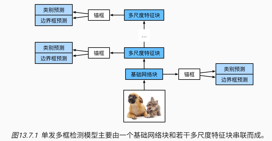
简言之，通过多尺度特征块，单发多框检测生成不同大小的锚框，并通过预测边界框的类别和偏移量来检测大小不同的目标，因此这是一个多尺度目标检测模型。

思考：特征图变量到锚框类别和偏移量的转换

给定形状为 $(B, C, H, W)$ 的特征图变量，其中 $B$ 、 $C$ 、 $H$ 和 $W$ 分别是特征图的批量大小、通道数、高度和宽度。怎样才能将这个变量转换为锚框类别和偏移量？输出的形状是什么？

思考：假设在特征图上的每一个像素格点生成 a 个锚框，分类任务的目标类别数（不含背景）为 q 类（因此含背景共q+1类）。

1. 形状转换逻辑与步骤

我们在特征图上需要预测两项内容：

类别：每个锚框需要预测 $q+1$ 个类别的概率；

偏移量：每个锚框预测需要4个位置偏移量 $(x, y, w, h)$ 。

转换过程通常采用：卷积 Conv 配合维度重排（Permute）与展平（Flatten）：

a) 用一个卷积层将通道数从 C 变换到对应的预测通道数。

b) 将输出维度 $(B,C,H,W)$ 调整为 $(B,H,W,C)$ ，使同一空间位置的预测值紧密相邻。

c) 将空间与锚框维度展平为一维向量，方便和 Ground Truth（真实框）计算损失函数。

2. 输出的形状：

类别： $\text{Shape}_{cls} = (B, \; H \times W \times a, \; q + 1)$ (或者展平为二维矩阵： $(B, \; H \times W \times a \times (q + 1))$ ）

偏移量： $\text{Shape}_{offset} = (B, \; H \times W \times a \times 4)$

—— 考虑输入和输入同一空间坐标 $(x,y)$ ：

输出特征图上 $(x,y)$ 坐标的通道里包含了以输入特征图上 $(x,y)$ 坐标为中心生成的所有锚框的类别预测。因此输出通道数为 $a \times (q + 1)$ ，其中索引为 $i(q + 1)+j(0\leq j\leq q)$ 的通道代表了索引为 $i$ 的锚框有关类别索引为 $j$ 的预测。

代码实现

1 模型定义

1.1 基础预测层与特征变换

1.1.2 核心转换模块实现

在SSD模型中，将特征图映射为锚框的预测类别与预测偏移的核心机制：

使用 $3\times 3$ 的 Conv，且padding=1，以保持宽高不变，使得输入和输出在特征图上的空间坐标一一对应，并将预测的通道数分别设为：

类别： $num_{anchors} \times (num_{classses} + 1)$
边界框： $num_{anchors} \times 4$

import torch
from torch import nn

def cls_predictor(num_inputs, num_anchors, num_classes):
    """ 类别预测层：输出通道数 = 锚框数 * (类别数 + 背景类1) """
    return nn.Conv2d(
        in_channels=num_inputs,
        out_channels=num_anchors * (num_classes + 1),
        kernel_size=3,
        padding=1
    )

def bbox_predictor(num_inputs, num_anchors):
    """ 边界框偏移量预测层：输出通道数 = 锚框数 * 4 个坐标偏移量 (x, y, w, h) """
    return nn.Conv2d(
        in_channels=num_inputs,
        out_channels=num_anchors * 4,
        kernel_size=3,
        padding=1
    )

1.1.2 维度重排与展平

由于SSD会在多个不同尺度的特征图上分别进行预测，而不同尺度下特征图的形状或以同一单元为中心的锚框的数量可能会有所不同。因此，不同尺度下预测出的形状可能会有所不同。

为了能将所有特征图的预测结果拼接在一起计算损失函数（Loss），我们需要将形状 $(B,C,H,W)$ 转换为 $(B,H*W*num_{anchors},num_{cls})$ 的统一二/三维格式。

def forward_prediction(x, block):
    """单层特征图的正向传播预测"""
    return block(x)

def flatten_pred(pred):
    """
    将 (Batch, Channel, Height, Width) 格式转换为 (Batch, Height * Width * Anchors, Num_Outputs)
    使得同一 Batch 内所有尺度的预测可以在 Dim=1 上进行拼接 (Concat)
    """
    # 1. 将通道维移动到最后：(B, C, H, W) -> (B, H, W, C)
    pred = pred.permute(0, 2, 3, 1)
    # 2. 从第1维开始展平：(B, H * W * C)
    return torch.flatten(pred, start_dim=1)

def concat_preds(preds):
    """将来自不同多尺度特征图的预测拼接在一起"""
    return torch.cat([flatten_pred(p) for p in preds], dim=1)

为什么 flatten_pred 里要用 .permute(0, 2, 3, 1)？

PyTorch 默认的特征图张量顺序是 (Batch, Channel, Height, Width)。对于分类层，假设通道数是 10，这意味着它连续排列了通道 $0\sim9$ 。如果不进行 permute 调整而直接展平（Flatten），不同网格格点（Height/Width）上的预测就会混在一起。先用 permute(0, 2, 3, 1) 把通道维调到最后变成 (Batch, Height, Width, Channel)，就能确保在展开时，同一个网格上的所有锚框预测数据在内存中是连续的。

1.1.3 多尺度输出拼接示例

# 假设参数设置
batch_size = 2
num_classes = 10  # 10 个真实类别（不含背景）
num_anchors = 5   # 每个格点生成 5 个锚框

# 假设来自网络的两个不同尺度特征图
# 特征图 1: 高分辨率 (针对小目标)，通道数 32
fmap1 = torch.zeros((batch_size, 32, 32, 32))  
# 特征图 2: 低分辨率 (针对大目标)，通道数 64
fmap2 = torch.zeros((batch_size, 64, 16, 16))  

# 为两个特征图定义对应的类别与偏移量预测器
cls_pred_1 = cls_predictor(32, num_anchors, num_classes)
cls_pred_2 = cls_predictor(64, num_anchors, num_classes)

bbox_pred_1 = bbox_predictor(32, num_anchors)
bbox_pred_2 = bbox_predictor(64, num_anchors)

# 1. 正向传播获取原生卷积预测输出
y1_cls = forward_prediction(fmap1, cls_pred_1)  # 形状: (2, 55, 32, 32)
y2_cls = forward_prediction(fmap2, cls_pred_2)  # 形状: (2, 55, 16, 16)

y1_bbox = forward_prediction(fmap1, bbox_pred_1) # 形状: (2, 20, 32, 32)
y2_bbox = forward_prediction(fmap2, bbox_pred_2) # 形状: (2, 20, 16, 16)

# 2. 展平并拼接多尺度预测
output_cls = concat_preds([y1_cls, y2_cls])
output_bbox = concat_preds([y1_bbox, y2_bbox])

print("类别预测最终输出形状:", output_cls.shape)
print("偏移量预测最终输出形状:", output_bbox.shape)

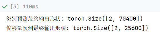
输出形状验证逻辑：

fmap1 锚框总数：32*32*5=5120； fmap 2 锚框总数：16*16*5=1280；

多尺度锚框总数：5120+1280=6400，因此打印结果

类别预测最终输出形状: $torch.Size([2, 70400]) (6400 \times 11)$

偏移量预测最终输出形状: $torch.Size([2, 25600]) (6400 \times 4)$

输出：

1.2 特征抽取基础模块

1.2.1 高宽减半特征抽取块

为了在多个尺度下检测目标，定义高宽减半模块，将输入特征图的高度和宽度减半。事实上，该块应用了在 subsec_vgg-blocks 中的VGG模块设计。
填充为1的3×3Conv不改变特征图的形状。但是，其后的2×2最大池化层将输入特征图的高度和宽度减少了一半。
对于此高和宽减半模块的输入和输出特征图，由于 $1\times 2+(3-1)+(3-1)=6$ ，所以输出中的每个单元在输入上都有一个 $6 \times 6$ 的感受野。因此，高宽减半模块会扩大每个单元在其输出特征图中的感受野。

[最终输出] 1 个点
    │
    ▼ (经过步幅=2的池化，1个点还原为 2x2 区域) ───> 1 × 2 = 2
[池化前]   2 x 2 的区域
    │
    ▼ (经过 3x3 卷积，边长扩展 3-1=2 格) ─────────> 2 + (3 - 1) = 4
[卷积2前]  4 x 4 的区域
    │
    ▼ (经过 3x3 卷积，边长再扩展 3-1=2 格) ───────> 4 + (3 - 1) = 6
[最初输入] 6 x 6 的区域！

def down_sample_blk(in_channels, out_channels):
    """高宽减半块：由两个 3x3 卷积 + BatchNorm + ReLU + 2x2 最大池化组成"""
    blk = []
    for _ in range(2):
        blk.append(nn.Conv2d(in_channels, out_channels, kernel_size=3, padding=1))
        blk.append(nn.BatchNorm2d(out_channels))
        blk.append(nn.ReLU())
        in_channels = out_channels
    blk.append(nn.MaxPool2d(2))
    return nn.Sequential(*blk)

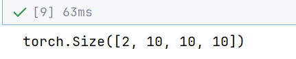
//示例：

forward_prediction(torch.zeros((2, 3, 20, 20)), down_sample_blk(3, 10)).shape

1.2.2 基础骨干网络

基本骨干网络用于从输入图像中抽取特征。为了计算简洁，构造一个小的基础网络，该网络串联3个高和宽减半块，并逐步将通道数翻倍。

def base_net():
    """基础网络 (Base Network)：连续 3 个高宽减半块，抽取基础特征图"""
    blk = []
    num_filters = [3, 16, 32, 64]
    for i in range(len(num_filters) - 1):
        blk.append(down_sample_blk(num_filters[i], num_filters[i + 1]))
    return nn.Sequential(*blk)

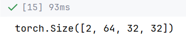
//示例：

给定输入图像的形状为 $256 \times 256$ ，此基本网络块输出的特征图形三次宽高减半为32。

1.3 完整TinySSD 模型定义

1.3.1 前置函数

完整的单发多框检测模型由5个模块组成：1*基本网络模块 + 3*高宽减半模块 + 最大池化。

def get_blk(i):
    if i == 0:
        blk = base_net()
    elif i == 1:
        blk = down_sample_blk(64, 128)
    elif i == 4:
        blk = nn.AdaptiveMaxPool2d((1,1))
    else:
        blk = down_sample_blk(128, 128)
    return blk

下面为每个模块定义前向传播。与图像分类任务不同，此处的输出包括：特征图Y＋根据Y生成的锚框+预测锚框的类别和偏移量。

def blk_forward(X, blk, size, ratio, cls_predictor, bbox_predictor):
    Y = blk(X)
    anchors = d2l.multibox_prior(Y, sizes=size, ratios=ratio)
    cls_preds = cls_predictor(Y)
    bbox_preds = bbox_predictor(Y)
    return (Y, anchors, cls_preds, bbox_preds)

一个接近顶部的多尺度特征块是用于检测较大目标定的，因此需要生成更大的锚框。在前向传播中，在每个多尺度特征块上，通过调用的multibox_prios函数的sizes参数传递两个比例值的列表。

sizes = [[0.2, 0.272], [0.37, 0.447], [0.54, 0.619], [0.71, 0.79],
         [0.88, 0.961]]
ratios = [[1, 2, 0.5]] * 5
num_anchors = len(sizes[0]) + len(ratios[0]) - 1

1.3.2 完整模型TinySSD

class TinySSD(nn.Module):
    def __init__(self, num_classes, **kwargs):
        super(TinySSD, self).__init__(**kwargs)
        self.num_classes = num_classes
        idx_to_in_channels = [64, 128, 128, 128, 128]
        for i in range(5):
            # 即赋值语句self.blk_i=get_blk(i)
            setattr(self, f'blk_{i}', get_blk(i))
            setattr(self, f'cls_{i}', cls_predictor(idx_to_in_channels[i],
                                                    num_anchors, num_classes))
            setattr(self, f'bbox_{i}', bbox_predictor(idx_to_in_channels[i],
                                                      num_anchors))

    def forward(self, X):
        anchors, cls_preds, bbox_preds = [None] * 5, [None] * 5, [None] * 5
        for i in range(5):
            # getattr(self,'blk_%d'%i)即访问self.blk_i
            X, anchors[i], cls_preds[i], bbox_preds[i] = blk_forward(
                X, getattr(self, f'blk_{i}'), sizes[i], ratios[i],
                getattr(self, f'cls_{i}'), getattr(self, f'bbox_{i}'))
        anchors = torch.cat(anchors, dim=1)
        cls_preds = concat_preds(cls_preds)
        cls_preds = cls_preds.reshape(
            cls_preds.shape[0], -1, self.num_classes + 1)
        bbox_preds = concat_preds(bbox_preds)
        return anchors, cls_preds, bbox_preds

//示例：

if __name__ == '__main__':
    # 示例参数配置：假设数据集有 1 个真实目标类别（如“狗”）
    net = TinySSD(num_classes=1)

    # 模拟输入一个图像 Batch：批大小为 2，3 通道，高宽均为 256
    X = torch.zeros((2, 3, 256, 256))

    # 前向传播预测
    anchors, cls_preds, bbox_preds = net(X)

    print("输入图像尺寸:", X.shape)
    print("类别预测输出尺寸 (Batch, 总锚框数, 类别数+1):", cls_preds.shape)
    print("偏移量预测输出尺寸 (Batch, 总锚框数 * 4):", bbox_preds.shape)

2 模型训练

2.1 读取数据集与初始化

from d2l import torch as d2l

batch_size = 32
train_iter, _ = d2l.load_data_bananas(batch_size)

初始化device、网络以及优化算法指定。

# 初始化参数以及优化算法
device, net = d2l.try_gpu(), TinySSD(num_classes=1)
trainer = torch.optim.SGD(net.parameters(), lr=0.2, weight_decay=5e-4)

2.2 损失函数与评价函数

（1）损失函数

目标检测有两种类型的损失。

锚框类别的损失（二分类）：可使用交叉熵损失函数计算。
锚框偏移量的损失（回归）：此处使用 $L_1$ 范数损失，即预测值和真实值之差的绝对值。

我们通过掩码变量 bbox_masks 使得负类锚框和填充锚框不参与损失的计算。最后，将锚框类别和偏移量的损失相加，以获得模型的最终损失函数。

# 类别损失
cls_loss = nn.CrossEntropyLoss(reduction='none')
# 偏移损失
bbox_loss = nn.L1Loss(reduction='none')

def calc_loss(cls_preds, cls_labels, bbox_preds, bbox_labels, bbox_masks):
    batch_size, num_classes = cls_preds.shape[0], cls_preds.shape[2]
    cls = cls_loss(cls_preds.reshape(-1, num_classes),
                   cls_labels.reshape(-1)).reshape(batch_size, -1).mean(dim=1)
    bbox = bbox_loss(bbox_preds * bbox_masks,
                     bbox_labels * bbox_masks).mean(dim=1)
    return cls + bbox

（2）评价函数

课程中沿用准确率评价分类结果。由于偏移量使用了 $L_1$ 范数损失，课程使用平均绝对误差来评价边界框的预测结果。这些预测结果是从生成的锚框及其预测偏移量中获得的。

def cls_eval(cls_preds, cls_labels):
    # 由于类别预测结果放在最后一维，argmax需要指定最后一维。
    return float((cls_preds.argmax(dim=-1).type(
        cls_labels.dtype) == cls_labels).sum())

def bbox_eval(bbox_preds, bbox_labels, bbox_masks):
    return float((torch.abs((bbox_labels - bbox_preds) * bbox_masks)).sum())

2.3 训练

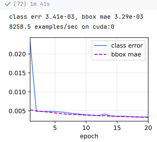
训练模型：在模型的前向传播过程中生成多尺度锚框（anchors），并预测其类别（cls_preds）和偏移量（bbox_preds）。然后，根据标签Y为生成的锚框标记类别（cls_labels）和偏移量（bbox_labels）。最后，根据类别和偏移量的预测和标注值计算损失函数。

num_epochs, timer = 20, d2l.Timer()
animator = d2l.Animator(xlabel='epoch', xlim=[1, num_epochs],
                        legend=['class error', 'bbox mae'])
net = net.to(device)
for epoch in range(num_epochs):
    # 训练精确度的和，训练精确度的和中的示例数
    # 绝对误差的和，绝对误差的和中的示例数
    metric = d2l.Accumulator(4)
    net.train()
    for features, target in train_iter:
        timer.start()
        trainer.zero_grad()
        X, Y = features.to(device), target.to(device)
        # 生成多尺度的锚框，为每个锚框预测类别和偏移量
        anchors, cls_preds, bbox_preds = net(X)
        # 为每个锚框标注类别和偏移量
        bbox_labels, bbox_masks, cls_labels = d2l.multibox_target(anchors, Y)
        # 根据类别和偏移量的预测和标注值计算损失函数
        l = calc_loss(cls_preds, cls_labels, bbox_preds, bbox_labels,
                      bbox_masks)
        l.mean().backward()
        trainer.step()
        metric.add(cls_eval(cls_preds, cls_labels), cls_labels.numel(),
                   bbox_eval(bbox_preds, bbox_labels, bbox_masks),
                   bbox_labels.numel())
    cls_err, bbox_mae = 1 - metric[0] / metric[1], metric[2] / metric[3]
    animator.add(epoch + 1, (cls_err, bbox_mae))
print(f'class err {cls_err:.2e}, bbox mae {bbox_mae:.2e}')
print(f'{len(train_iter.dataset) / timer.stop():.1f} examples/sec on '
      f'{str(device)}')

//输出：

3 模型预测

读取图像，将其转换成卷积层需要的4维格式。

import torchvision
X = torchvision.io.read_image('data/banana-detection/bananas_val/images/0.png').unsqueeze(0).float()
img = X.squeeze(0).permute(1, 2, 0).long()

multibox_detection函数：可以根据锚框及其预测偏移量得到预测边界框。然后，通过非极大值抑制来移除相似的预测边界框。

from torch.nn import functional as F

def predict(X):
    "预测-检测目标"
    net.eval()
    anchors, cls_preds, bbox_preds = net(X.to(device))
    cls_probs = F.softmax(cls_preds, dim=2).permute(0, 2, 1)
    output = d2l.multibox_detection(cls_probs, bbox_preds, anchors)
    idx = [i for i, row in enumerate(output[0]) if row[0] != -1]
    return output[0, idx]

output = predict(X)

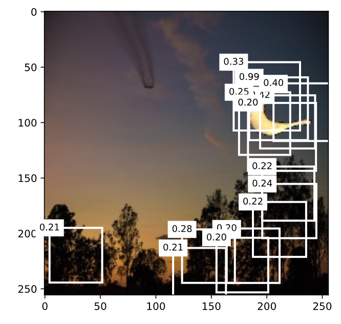
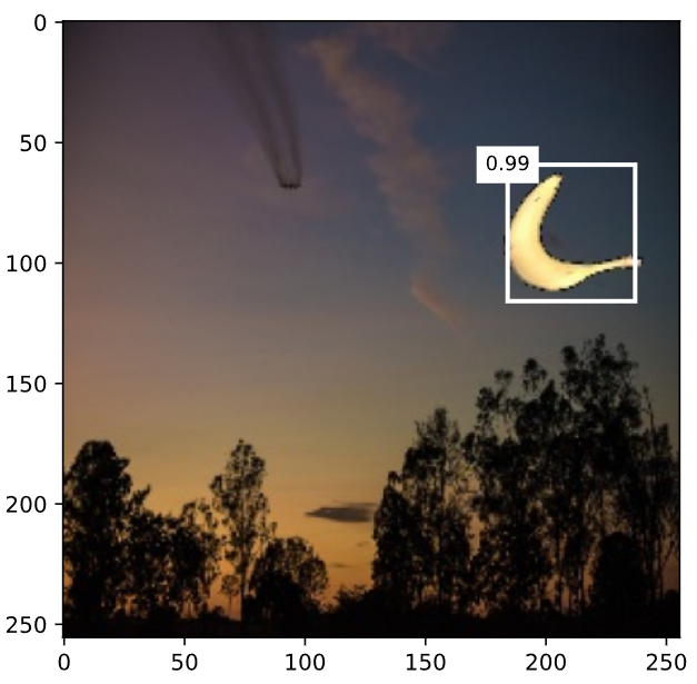
下面查看置信度阈值分别为0.2 和 0.9 的输出结果：

def display(img, output, threshold):
    d2l.set_figsize((5, 5))
    fig = d2l.plt.imshow(img)
    for row in output:
        score = float(row[1])
        if score < threshold:
            continue
        h, w = img.shape[0:2]
        bbox = [row[2:6] * torch.tensor((w, h, w, h), device=row.device)]
        d2l.show_bboxes(fig.axes, bbox, '%.2f' % score, 'w')

display(img, output.cpu(), threshold=0.2)