● 🍨 本文为🔗365天深度学习训练营中的学习记录博客
● 🍖 原作者：K同学啊

学习目标：

1.本地加载数据。

2.测试集accuracy达到93%

一、前期准备

1.设置GPU

import torch
import torch.nn as nn
import torchvision.transforms as transforms
import torchvision
from torchvision import transforms, datasets
import os,PIL,pathlib,random

device = torch.device("cuda" if torch.cuda.is_available() else "cpu")
device

2.导入数据

把天气数据集命名为data，其下有四个文件夹（cloudy，rain，shine，sunrise），储存不同天气的照片，把data文件夹

和代码文件放在同一目录下

data_dir = './data/'
data_dir = pathlib.Path(data_dir)

data_paths = list(data_dir.glob('*'))
classeNames = [str(path).split("\\")[1] for path in data_paths]
classeNames

import matplotlib.pyplot as plt
from PIL import Image

# 指定图像文件夹路径
image_folder = './data/cloudy/'

# 获取文件夹中的所有图像文件
image_files = [f for f in os.listdir(image_folder) if f.endswith((".jpg", ".png", ".jpeg"))]

fig, axes = plt.subplots(3, 8, figsize=(16, 6))

# 使用列表推导式加载和显示图像
for ax, img_file in zip(axes.flat, image_files):
    img_path = os.path.join(image_folder, img_file)
    img = Image.open(img_path)
    ax.imshow(img)
    ax.axis('off')

# 显示图像
plt.tight_layout()
plt.show()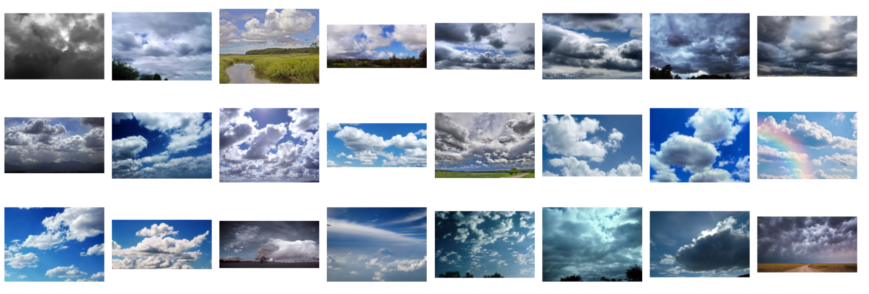

total_datadir = './data/'

# 关于transforms.Compose的更多介绍可以参考：https://blog.csdn.net/qq_38251616/article/details/124878863
train_transforms = transforms.Compose([
    transforms.Resize([224, 224]),  # 将输入图片resize成统一尺寸
    transforms.ToTensor(),          # 将PIL Image或numpy.ndarray转换为tensor，并归一化到[0,1]之间
    transforms.Normalize(           # 标准化处理-->转换为标准正太分布（高斯分布），使模型更容易收敛
        mean=[0.485, 0.456, 0.406], 
        std=[0.229, 0.224, 0.225])  # 其中 mean=[0.485,0.456,0.406]与std=[0.229,0.224,0.225] 从数据集中随机抽样计算得到的。
])

total_data = datasets.ImageFolder(total_datadir,transform=train_transforms)
total_data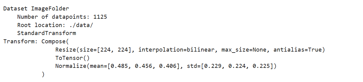

3.划分数据集

train_size = int(0.8 * len(total_data))
test_size  = len(total_data) - train_size
train_dataset, test_dataset = torch.utils.data.random_split(total_data, [train_size, test_size])
train_dataset, test_dataset

train_size,test_size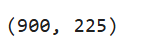

batch_size = 32

train_dl = torch.utils.data.DataLoader(train_dataset,
                                       batch_size=batch_size,
                                       shuffle=True)
test_dl = torch.utils.data.DataLoader(test_dataset,
                                      batch_size=batch_size,
                                      shuffle=True)
for X, y in test_dl:
    print("Shape of X [N, C, H, W]: ", X.shape)
    print("Shape of y: ", y.shape, y.dtype)
    break

二、构建CNN网络

import torch.nn.functional as F

class Network_bn(nn.Module):
    def __init__(self):
        super(Network_bn, self).__init__()
        """
        nn.Conv2d()函数：
        第一个参数（in_channels）是输入的channel数量
        第二个参数（out_channels）是输出的channel数量
        第三个参数（kernel_size）是卷积核大小
        第四个参数（stride）是步长，默认为1
        第五个参数（padding）是填充大小，默认为0
        """
        self.conv1 = nn.Conv2d(in_channels=3, out_channels=12, kernel_size=5, stride=1, padding=0)
        self.bn1 = nn.BatchNorm2d(12)
        self.conv2 = nn.Conv2d(in_channels=12, out_channels=12, kernel_size=5, stride=1, padding=0)
        self.bn2 = nn.BatchNorm2d(12)
        self.pool1 = nn.MaxPool2d(2,2)
        self.conv4 = nn.Conv2d(in_channels=12, out_channels=24, kernel_size=5, stride=1, padding=0)
        self.bn4 = nn.BatchNorm2d(24)
        self.conv5 = nn.Conv2d(in_channels=24, out_channels=24, kernel_size=5, stride=1, padding=0)
        self.bn5 = nn.BatchNorm2d(24)
        self.pool2 = nn.MaxPool2d(2,2)
        self.fc1 = nn.Linear(24*50*50, len(classeNames))

    def forward(self, x):
        x = F.relu(self.bn1(self.conv1(x)))      
        x = F.relu(self.bn2(self.conv2(x)))     
        x = self.pool1(x)                        
        x = F.relu(self.bn4(self.conv4(x)))     
        x = F.relu(self.bn5(self.conv5(x)))  
        x = self.pool2(x)                        
        x = x.view(-1, 24*50*50)
        x = self.fc1(x)

        return x

device = "cuda" if torch.cuda.is_available() else "cpu"
print("Using {} device".format(device))

model = Network_bn().to(device)
model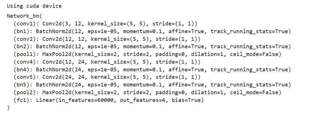

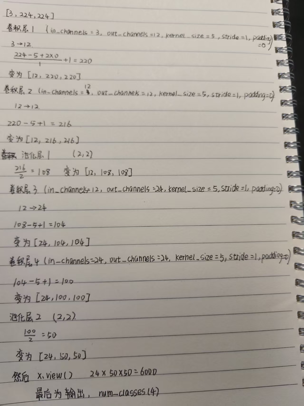
卷积层和池化层的计算

三、训练模型

1.设置超参数

loss_fn    = nn.CrossEntropyLoss() # 创建损失函数
learn_rate = 1e-4 # 学习率
opt        = torch.optim.SGD(model.parameters(),lr=learn_rate)

2.编写训练函数

# 训练循环
def train(dataloader, model, loss_fn, optimizer):
    size = len(dataloader.dataset)  # 训练集的大小，一共60000张图片
    num_batches = len(dataloader)   # 批次数目，1875（60000/32）

    train_loss, train_acc = 0, 0  # 初始化训练损失和正确率
    
    for X, y in dataloader:  # 获取图片及其标签
        X, y = X.to(device), y.to(device)
        
        # 计算预测误差
        pred = model(X)          # 网络输出
        loss = loss_fn(pred, y)  # 计算网络输出和真实值之间的差距，targets为真实值，计算二者差值即为损失
        
        # 反向传播
        optimizer.zero_grad()  # grad属性归零
        loss.backward()        # 反向传播
        optimizer.step()       # 每一步自动更新
        
        # 记录acc与loss
        train_acc  += (pred.argmax(1) == y).type(torch.float).sum().item()
        train_loss += loss.item()
            
    train_acc  /= size
    train_loss /= num_batches

    return train_acc, train_loss

3.编写测试函数

def test (dataloader, model, loss_fn):
    size        = len(dataloader.dataset)  # 测试集的大小，一共10000张图片
    num_batches = len(dataloader)          # 批次数目，313（10000/32=312.5，向上取整）
    test_loss, test_acc = 0, 0
    
    # 当不进行训练时，停止梯度更新，节省计算内存消耗
    with torch.no_grad():
        for imgs, target in dataloader:
            imgs, target = imgs.to(device), target.to(device)
            
            # 计算loss
            target_pred = model(imgs)
            loss        = loss_fn(target_pred, target)
            
            test_loss += loss.item()
            test_acc  += (target_pred.argmax(1) == target).type(torch.float).sum().item()

    test_acc  /= size
    test_loss /= num_batches

    return test_acc, test_loss

4.正式训练

epochs     = 20
train_loss = []
train_acc  = []
test_loss  = []
test_acc   = []

for epoch in range(epochs):
    model.train()
    epoch_train_acc, epoch_train_loss = train(train_dl, model, loss_fn, opt)
    
    model.eval()
    epoch_test_acc, epoch_test_loss = test(test_dl, model, loss_fn)
    
    train_acc.append(epoch_train_acc)
    train_loss.append(epoch_train_loss)
    test_acc.append(epoch_test_acc)
    test_loss.append(epoch_test_loss)
    
    template = ('Epoch:{:2d}, Train_acc:{:.1f}%, Train_loss:{:.3f}, Test_acc:{:.1f}%，Test_loss:{:.3f}')
    print(template.format(epoch+1, epoch_train_acc*100, epoch_train_loss, epoch_test_acc*100, epoch_test_loss))
print('Done')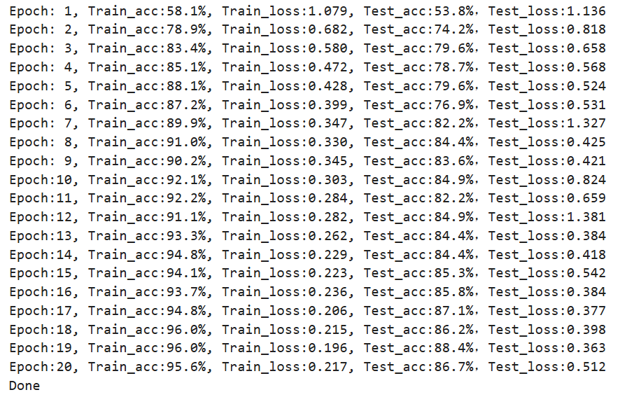

五、结果可视化

import matplotlib.pyplot as plt
#隐藏警告
import warnings
warnings.filterwarnings("ignore")               #忽略警告信息
plt.rcParams['font.sans-serif']    = ['SimHei'] # 用来正常显示中文标签
plt.rcParams['axes.unicode_minus'] = False      # 用来正常显示负号
plt.rcParams['figure.dpi']         = 100        #分辨率

from datetime import datetime
current_time = datetime.now() # 获取当前时间

epochs_range = range(epochs)

plt.figure(figsize=(12, 3))
plt.subplot(1, 2, 1)

plt.plot(epochs_range, train_acc, label='Training Accuracy')
plt.plot(epochs_range, test_acc, label='Test Accuracy')
plt.legend(loc='lower right')
plt.title('Training and Validation Accuracy')
plt.xlabel(current_time) 

plt.subplot(1, 2, 2)
plt.plot(epochs_range, train_loss, label='Training Loss')
plt.plot(epochs_range, test_loss, label='Test Loss')
plt.legend(loc='upper right')
plt.title('Training and Validation Loss')
plt.show()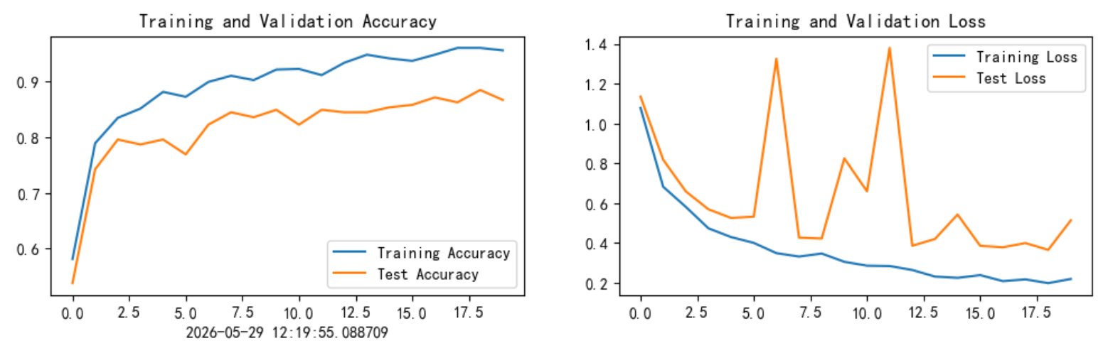

六、模型调优

为了提高准确率，我改变了优化器的参数，为SGD添加动量（momentum），使用余弦退火调度器，让学习率平滑从高到低。

loss_fn    = nn.CrossEntropyLoss() # 创建损失函数
opt        = torch.optim.SGD(model.parameters(),lr=0.001,momentum=0.9)
scheduler = torch.optim.lr_scheduler.CosineAnnealingLR(opt,T_max=20,eta_min=1e-5)

把scheduler.step()放在正式训练epoch循环的末尾，让学习率逐渐降低

epochs     = 20
train_loss = []
train_acc  = []
test_loss  = []
test_acc   = []

for epoch in range(epochs):
    model.train()
    epoch_train_acc, epoch_train_loss = train(train_dl, model, loss_fn, opt)
    
    model.eval()
    epoch_test_acc, epoch_test_loss = test(test_dl, model, loss_fn)
    
    train_acc.append(epoch_train_acc)
    train_loss.append(epoch_train_loss)
    test_acc.append(epoch_test_acc)
    test_loss.append(epoch_test_loss)
    
    template = ('Epoch:{:2d}, Train_acc:{:.1f}%, Train_loss:{:.3f}, Test_acc:{:.1f}%，Test_loss:{:.3f}')
    print(template.format(epoch+1, epoch_train_acc*100, epoch_train_loss, epoch_test_acc*100, epoch_test_loss))
    scheduler.step()#在这里添加，使得每轮的学习率逐渐降低
print('Done')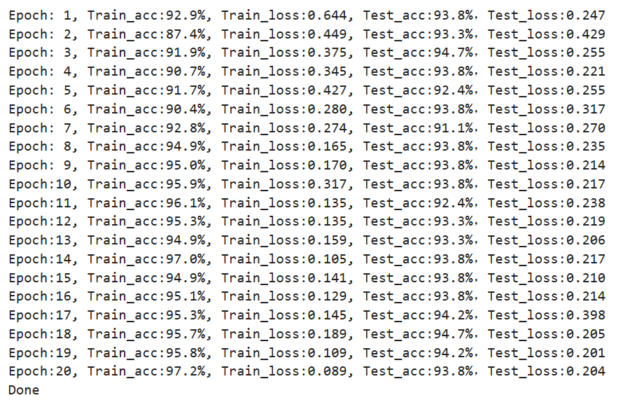

此时准确率达到93%

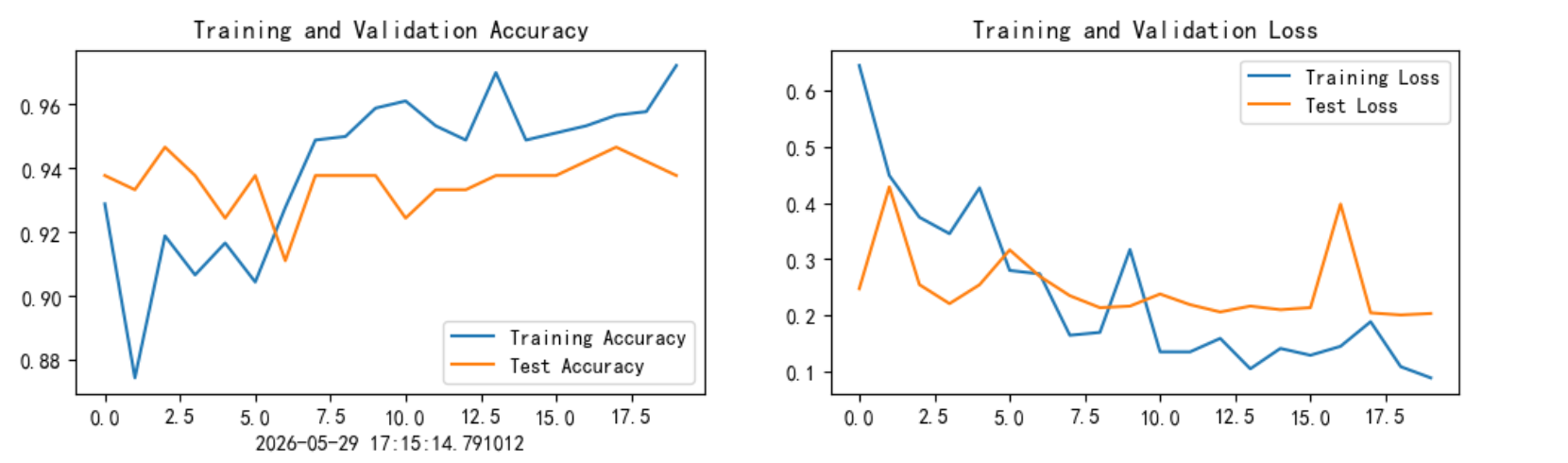
个人总结：这次为了达到测试集准确率的标准，在调整模型的过程中我试过用余弦退火和warmup的方式调节学习率，并对优化器的参数做了很多次改变，试过Adam和SGD，也尝试在模型中添加dropout层，最终用上述方法达到了93%，但是这个准确率也可能具有偶然性，不能每次都达到，后续我再做其他调整也没有办法让准确率达到95%，通过这次模型调优，我对优化器，学习率等有了更深的理解。