
P6:VGG-16算法-Pytorch实现人脸识别
- 🍨 本文为🔗365天深度学习训练营中的学习记录博客
- 🍖 原作者:K同学啊
学习目的:
- 保存训练过程中的最佳模型权重
- 调用官方的VGG-16网络框架
一、 前期准备
关于环境
- 语言环境:Python3.13
- 编译器:vsCode
- 深度学习环境:torch==2.11.0+cu130;torchvision==0.26.0+cu130torchvision==0.26.0+cu130
1.设置GPU
设置分析环境:
import torch
import torch.nn as nn
import torchvision.transforms as transforms
import torchvision
from torchvision import transforms, datasets
import os,PIL,pathlib,warnings

warnings.filterwarnings("ignore")             #忽略警告信息

device = torch.device("cuda" if torch.cuda.is_available() else "cpu")
device
运行结果:

2. 导入数据
由于本次是本地数据,因此不需要有download代码,只需读取路径里的数据集即可
import os,PIL,random,pathlib

data_dir = './48-data/'
data_dir = pathlib.Path(data_dir)

data_paths  = list(data_dir.glob('*'))
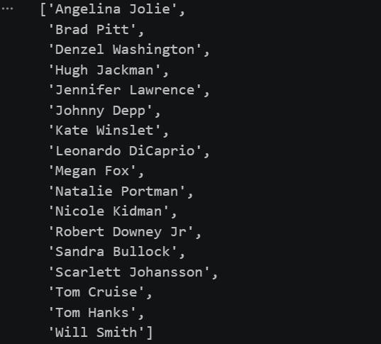
classeNames = [str(path).split("\\")[1] for path in data_paths]
classeNames
运行结果:
3.图片预处理
# 关于transforms.Compose的更多介绍可以参考:https://blog.csdn.net/qq_38251616/article/details/124878863
train_transforms = transforms.Compose([
    transforms.Resize([224, 224]),  # 将输入图片resize成统一尺寸
    # transforms.RandomHorizontalFlip(), # 随机水平翻转
    transforms.ToTensor(),          # 将PIL Image或numpy.ndarray转换为tensor,并归一化到[0,1]之间
    transforms.Normalize(           # 标准化处理-->转换为标准正太分布(高斯分布),使模型更容易收敛
        mean=[0.485, 0.456, 0.406],
        std=[0.229, 0.224, 0.225])  # 其中 mean=[0.485,0.456,0.406]与std=[0.229,0.224,0.225] 从数据集中随机抽样计算得到的。
])

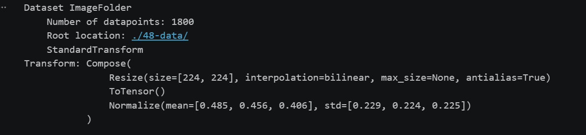
total_data = datasets.ImageFolder("./48-data/",transform=train_transforms)
total_data
代码解读:
在进行图片识别前,为提高模型的泛化能力,一般要对图片进行统一的预处理 以保证图片的基本格式一致:
模型要求输入尺寸一致 → Resize。
PyTorch 模型要求输入是张量 → ToTensor。
标准化有助于模型更快收敛 → Normalize。
mean与std数值是怎么来的?
这些均值和标准差是通过计算ImageNet数据集中所有训练图像的RGB通道均值和标准差得出的。具体计算过程如下:
获取ImageNet数据集:每张图像通常具有RGB三个通道。
计算均值(Mean):
遍历所有图像,分别计算每个通道(R、G、B)的像素值平均值,得到:
Red 通道均值 ≈ 0.485
Green 通道均值 ≈ 0.456
Blue 通道均值 ≈ 0.406
计算标准差(Standard Deviation):
遍历所有图像,计算每个通道的像素值标准差,得到:
Red 通道标准差 ≈ 0.229
Green 通道标准差 ≈ 0.224
Blue 通道标准差 ≈ 0.225
运行结果:
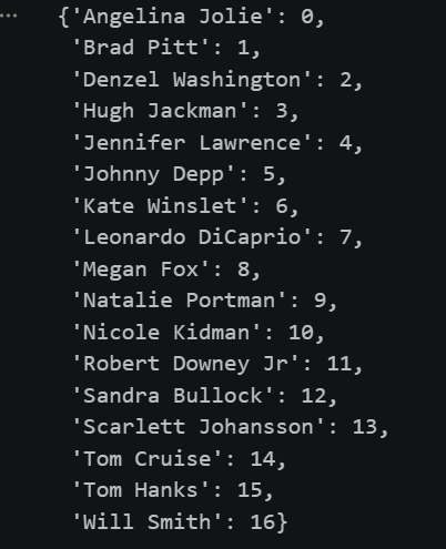
total_data.class_to_idx代码解读:
total_data.class_to_idx是一个存储了数据集类别和对应索引的字典。在PyTorch的ImageFolder数据加载器中,根据数据集文件夹的组织结构,每个文件夹代表一个类别,class_to_idx字典将每个类别名称映射为一个数字索引。此处打印出每个明星名字对应的数字标签(从 0 到 16)
运行结果:
4. 划分数据集
train_size = int(0.8 * len(total_data))
test_size  = len(total_data) - train_size
train_dataset, test_dataset = torch.utils.data.random_split(total_data, [train_size, test_size])
train_dataset, test_dataset
代码运行结果:

batch_size = 32

train_dl = torch.utils.data.DataLoader(train_dataset,
                                           batch_size=batch_size,
                                           shuffle=True,
                                           num_workers=1)
test_dl = torch.utils.data.DataLoader(test_dataset,
                                          batch_size=batch_size,
                                          shuffle=True,
                                          num_workers=1)
代码解读:
DataLoader将数据集包装成可迭代的批次。
batch_size=32:每批取 32 张图片,同时训练或测试,提高效率。
shuffle=True:训练时打乱数据顺序,增加随机性,防止模型记住顺序。
num_workers=1:用 1 个子进程加载数据(可加速 I/O)。
for X, y in test_dl:
    print("Shape of X [N, C, H, W]: ", X.shape)
    print("Shape of y: ", y.shape, y.dtype)
    break
代码运行结果:

查看一个批次的数据形状:
X是图像张量,形状为[32, 3, 224, 224](32 张,3 通道,高宽 224);y是标签,形状为[32],类型为torch.int64。
二、调用官方的VGG-16模型
VGG-16(Visual Geometry Group-16)是由牛津大学视觉几何组(Visual Geometry Group)提出的一种深度卷积神经网络架构,用于图像分类和对象识别任务。
模型架构:
- 13个卷积层(Convolutional Layer),分别用
blockX_convX表示;- 3个全连接层(Fully connected Layer),用
classifier表示;- 5个池化层(Pool layer)。
1.调用模型
from torchvision.models import vgg16

device = "cuda" if torch.cuda.is_available() else "cpu"
print("Using {} device".format(device))

# 加载预训练模型,并且对模型进行微调
model = vgg16(pretrained = True).to(device) # 加载预训练的vgg16模型

for param in model.parameters():
    param.requires_grad = False # 冻结模型的参数,这样子在训练的时候只训练最后一层的参数

# 修改classifier模块的第6层(即:(6): Linear(in_features=4096, out_features=2, bias=True))
# 注意查看我们下方打印出来的模型
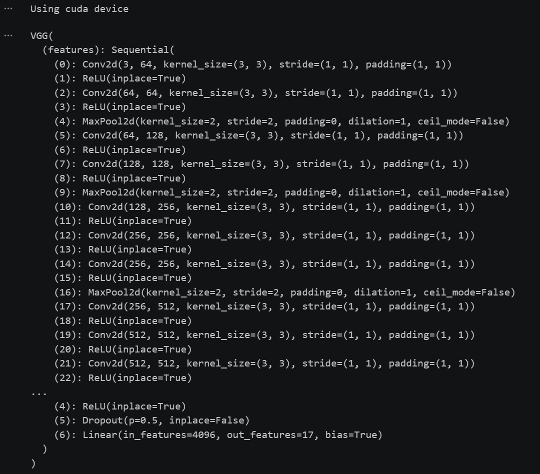
model.classifier._modules['6'] = nn.Linear(4096,len(classeNames)) # 修改vgg16模型中最后一层全连接层,输出目标类别个数
model.to(device)
model
代码解读:
vgg16(pretrained=True):加载在 ImageNet 上预训练好的 VGG16 模型,它已经学会了提取图像特征的能力。冻结参数:
param.requires_grad = False,这样在训练时,前面的卷积层参数不会更新,只更新后面新加的层的参数。这叫迁移学习,好处是:我们的数据量较小,直接用预训练特征,只需微调最后的分类层。修改最后一层:原 VGG16 最后一层输出是 1000 类(ImageNet 类别数),我们把它替换成一个输出为 17 类的线性层(全连接层)。
model.classifier._modules['6']定位到分类器的第 6 层(索引从 0 开始),将其替换为新的线性层。最后将模型移到 GPU(如果可用)。
代码运行结果:
三、 训练模型
1. 编写训练函数
def train(dataloader, model, loss_fn, optimizer):
    size = len(dataloader.dataset)  # 训练集的大小
    num_batches = len(dataloader)   # 批次数目, (size/batch_size,向上取整)

    train_loss, train_acc = 0, 0  # 初始化训练损失和正确率

    for X, y in dataloader:  # 获取图片及其标签
        X, y = X.to(device), y.to(device)

        # 计算预测误差
        pred = model(X)          # 网络输出
        loss = loss_fn(pred, y)  # 计算网络输出和真实值之间的差距,targets为真实值,计算二者差值即为损失

        # 反向传播
        optimizer.zero_grad()  # grad属性归零
        loss.backward()        # 反向传播
        optimizer.step()       # 每一步自动更新

        # 记录acc与loss
        train_acc  += (pred.argmax(1) == y).type(torch.float).sum().item()
        train_loss += loss.item()

    train_acc  /= size
    train_loss /= num_batches

    return train_acc, train_loss
2. 编写测试函数
测试函数和训练函数大致相同,但是由于不进行梯度下降对网络权重进行更新,所以不需要传入优化器
def test (dataloader, model, loss_fn):
    size        = len(dataloader.dataset)  # 测试集的大小
    num_batches = len(dataloader)          # 批次数目, (size/batch_size,向上取整)
    test_loss, test_acc = 0, 0

    # 当不进行训练时,停止梯度更新,节省计算内存消耗
    with torch.no_grad():
        for imgs, target in dataloader:
            imgs, target = imgs.to(device), target.to(device)

            # 计算loss
            target_pred = model(imgs)
            loss        = loss_fn(target_pred, target)

            test_loss += loss.item()
            test_acc  += (target_pred.argmax(1) == target).type(torch.float).sum().item()

    test_acc  /= size
    test_loss /= num_batches

    return test_acc, test_loss
3. 设置动态学习率
# 调用官方动态学习率接口时使用
learn_rate = 1e-4 # 初始学习率
lambda1 = lambda epoch: 0.92 ** (epoch // 4)
optimizer = torch.optim.SGD(model.parameters(), lr=learn_rate)
scheduler = torch.optim.lr_scheduler.LambdaLR(optimizer, lr_lambda=lambda1) #选定调整方法
代码解读:
optimizer:随机梯度下降(SGD),学习率初始为 0.0001。
scheduler:学习率调度器,按照lambda1函数调整学习率:每 4 个 epoch,学习率乘以 0.92。这样学习率会逐渐减小,有助于模型收敛。
4. 正式训练
import copy

loss_fn    = nn.CrossEntropyLoss() # 创建损失函数
epochs     = 40

train_loss = []
train_acc  = []
test_loss  = []
test_acc   = []

best_acc = 0    # 设置一个最佳准确率,作为最佳模型的判别指标

for epoch in range(epochs):
    # 更新学习率(使用自定义学习率时使用)
    # adjust_learning_rate(optimizer, epoch, learn_rate)

    model.train()
    epoch_train_acc, epoch_train_loss = train(train_dl, model, loss_fn, optimizer)
    scheduler.step() # 更新学习率(调用官方动态学习率接口时使用)

    model.eval()
    epoch_test_acc, epoch_test_loss = test(test_dl, model, loss_fn)

    # 保存最佳模型到 best_model
    if epoch_test_acc > best_acc:
        best_acc   = epoch_test_acc
        best_model = copy.deepcopy(model)

    train_acc.append(epoch_train_acc)
    train_loss.append(epoch_train_loss)
    test_acc.append(epoch_test_acc)
    test_loss.append(epoch_test_loss)

    # 获取当前的学习率
    lr = optimizer.state_dict()['param_groups'][0]['lr']

    template = ('Epoch:{:2d}, Train_acc:{:.1f}%, Train_loss:{:.3f}, Test_acc:{:.1f}%, Test_loss:{:.3f}, Lr:{:.2E}')
    print(template.format(epoch+1, epoch_train_acc*100, epoch_train_loss,
                          epoch_test_acc*100, epoch_test_loss, lr))

# 保存最佳模型到文件中
PATH = './best_model.pth'  # 保存的参数文件名
torch.save(best_model.state_dict(), PATH)

print('Done')
代码解读:
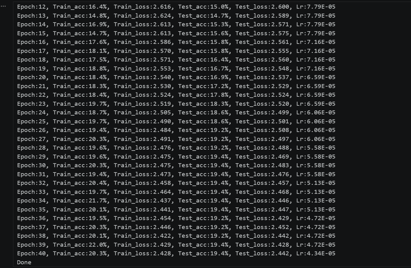
代码运行结果:
四、 结果可视化
1. Loss与Accuracy图
import matplotlib.pyplot as plt
#隐藏警告
import warnings
warnings.filterwarnings("ignore")               #忽略警告信息
plt.rcParams['font.sans-serif']    = ['SimHei'] # 用来正常显示中文标签
plt.rcParams['axes.unicode_minus'] = False      # 用来正常显示负号
plt.rcParams['figure.dpi']         = 100        #分辨率

from datetime import datetime
current_time = datetime.now() # 获取当前时间

epochs_range = range(epochs)

plt.figure(figsize=(12, 3))
plt.subplot(1, 2, 1)

plt.plot(epochs_range, train_acc, label='Training Accuracy')
plt.plot(epochs_range, test_acc, label='Test Accuracy')
plt.legend(loc='lower right')
plt.title('Training and Validation Accuracy')
plt.xlabel(current_time) # 打卡请带上时间戳,否则代码截图无效

plt.subplot(1, 2, 2)
plt.plot(epochs_range, train_loss, label='Training Loss')
plt.plot(epochs_range, test_loss, label='Test Loss')
plt.legend(loc='upper right')
plt.title('Training and Validation Loss')
plt.show()
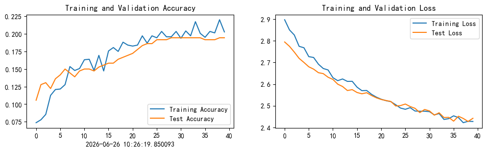
代码运行结果:
五、手动搭建VGG-16网络框架
import torch.nn.functional as F

class Model(nn.Module):
    def __init__(self):
        super(Model, self).__init__()
        self.conv1=nn.Sequential(
            nn.Conv2d(3, 64, kernel_size=3, padding=1), # 64*224*224
            nn.ReLU(inplace=True))

        self.conv2=nn.Sequential(
            nn.Conv2d(64, 64, kernel_size=3, padding=1), # 64*224*224
            nn.ReLU(inplace=True))

        self.pool1=nn.Sequential(
            nn.MaxPool2d(kernel_size=2, stride=2))       # 64*112*112

        self.conv3=nn.Sequential(
            nn.Conv2d(64, 128, kernel_size=3, padding=1), # 128*112*112
            nn.ReLU(inplace=True))

        self.conv4=nn.Sequential(
            nn.Conv2d(128, 128, kernel_size=3, padding=1), # 128*112*112
            nn.ReLU(inplace=True))

        self.pool2=nn.Sequential(
            nn.MaxPool2d(kernel_size=2, stride=2))         # 128*56*56

        self.conv5=nn.Sequential(
            nn.Conv2d(128, 256, kernel_size=3, padding=1), # 256*56*56
            nn.ReLU(inplace=True))

        self.conv6=nn.Sequential(
            nn.Conv2d(256, 256, kernel_size=3, padding=1), # 256*56*56
            nn.ReLU(inplace=True))

        self.conv7=nn.Sequential(
            nn.Conv2d(256, 256, kernel_size=3, padding=1), # 256*56*56
            nn.ReLU(inplace=True))

        self.pool3=nn.Sequential(
            nn.MaxPool2d(kernel_size=2, stride=2))         # 256*28*28

        self.conv8=nn.Sequential(
            nn.Conv2d(256, 512, kernel_size=3, padding=1), # 512*28*28
            nn.ReLU(inplace=True))

        self.conv9=nn.Sequential(
            nn.Conv2d(512, 512, kernel_size=3, padding=1), # 256*28*28
            nn.ReLU(inplace=True))

        self.conv10=nn.Sequential(
            nn.Conv2d(512, 512, kernel_size=3, padding=1), # 28*28*512
            nn.ReLU(inplace=True))

        self.pool4=nn.Sequential(
            nn.MaxPool2d(kernel_size=2, stride=2))         # 512*14*14

        self.conv11=nn.Sequential(
            nn.Conv2d(512, 512, kernel_size=3, padding=1), # 512*14*14
            nn.ReLU(inplace=True))

        self.conv12=nn.Sequential(
            nn.Conv2d(512, 512, kernel_size=3, padding=1), # 512*14*14
            nn.ReLU(inplace=True))

        self.conv13=nn.Sequential(
            nn.Conv2d(512, 512, kernel_size=3, padding=1), # 512*14*14
            nn.ReLU(inplace=True))

        self.pool5=nn.Sequential(
            nn.MaxPool2d(kernel_size=2, stride=2))         #  512*7*7

        self.avgpool = nn.AdaptiveAvgPool2d((7, 7))
        self.classifier = nn.Sequential(
            nn.Linear(512*7*7, 4096),  # 输入是展平后的特征向量 (25088)
            nn.ReLU(inplace=True),
            nn.Dropout(p=0.5),
            nn.Linear(4096, 4096),
            nn.ReLU(inplace=True),
            nn.Dropout(p=0.5),
            nn.Linear(4096, 1000),  # 默认输出1000个ImageNet类别
)

    def forward(self, x):

        batch_size = x.size(0)
        x = self.conv1(x)  # 卷积-BN-激活
        x = self.conv2(x)  # 卷积-BN-激活
        x = self.pool1(x)  # 池化
        x = self.conv3(x)  # 卷积-BN-激活
        x = self.conv4(x)  # 卷积-BN-激活
        x = self.pool2(x)  # 池化
        x = self.conv5(x)  # 卷积-激活
        x = self.conv6(x)  # 卷积-激活
        x = self.conv7(x)  # 卷积-激活
        x = self.pool3(x)  # 池化
        x = self.conv8(x)  # 卷积-激活
        x = self.conv9(x)  # 卷积-激活
        x = self.conv10(x) # 卷积-激活
        x = self.pool4(x)  # 池化
        x = self.conv11(x) # 卷积-激活
        x = self.conv12(x) # 卷积-激活
        x = self.conv13(x) # 卷积-激活
        x = self.pool5(x)  # 池化
        x = self.avgpool(x)
        x = x.view(batch_size, -1)
        x = self.dropout(x)
        x = self.fc(x)

        return x
六、提升模型效能
提升模型效能方法:
解冻部分卷积层进行微调(fine-tune),让网络适应人脸数据。
增加数据增强(随机水平翻转、随机旋转、颜色抖动等)以增加数据多样性。
调整学习率、优化器(比如Adam)。
增加训练轮数。
使用更深的网络(如ResNet)或更大的预训练模型。
检查数据标签是否正确,类别是否均衡。
使用更合适的损失函数或类别权重(如果类别不平衡)。
尝试对模块5进行解冻后训练
from torchvision.models import vgg16

device = "cuda" if torch.cuda.is_available() else "cpu"
print("Using {} device".format(device))

# 加载预训练模型,并且对模型进行微调
model = vgg16(pretrained = True).to(device) # 加载预训练的vgg16模型

for param in model.parameters():
    param.requires_grad = False # 冻结模型的参数,这样子在训练的时候只训练最后一层的参数

# 解冻 block5 的卷积层(在 features 中的索引 24~29)
for i in range(24, 30):   # 根据你的模型打印出的索引调整
    for param in model.features[i].parameters():
        param.requires_grad = True
# 修改classifier模块的第6层(即:(6): Linear(in_features=4096, out_features=2, bias=True))
# 注意查看我们下方打印出来的模型
model.classifier._modules['6'] = nn.Linear(4096,len(classeNames)) # 修改vgg16模型中最后一层全连接层,输出目标类别个数
model.to(device)
model
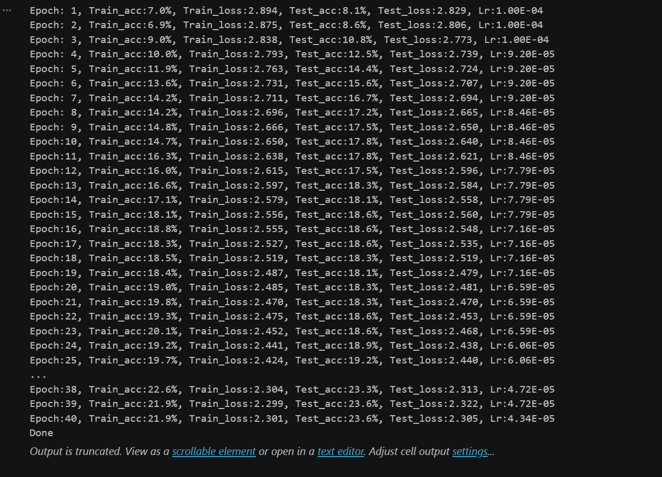
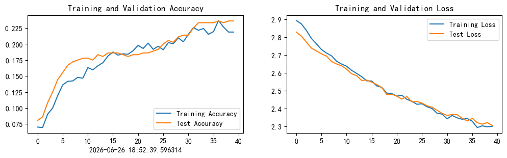
运行结果
模型准确率提升至23%,但远未达60%
对单张图片预测:
from PIL import Image

classes = list(total_data.class_to_idx)

def predict_one_image(image_path, model, transform, classes):

    test_img = Image.open(image_path).convert('RGB')
    plt.imshow(test_img)  # 展示预测的图片

    test_img = transform(test_img)
    img = test_img.to(device).unsqueeze(0)

    model.eval()
    output = model(img)

    _,pred = torch.max(output,1)
    pred_class = classes[pred]
    print(f'预测结果是:{pred_class}')
# 预测训练集中的某张照片
predict_one_image(image_path='./48-data/Angelina Jolie/001_fe3347c0.jpg',
model=model,
transform=train_transforms,
classes=classes)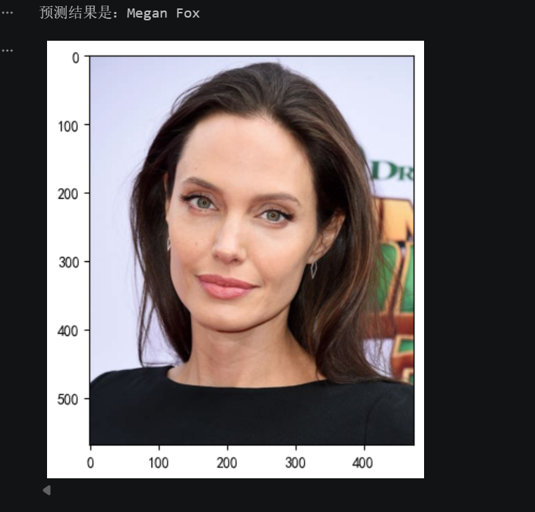
七、感悟
本周学习的是调用预训练模型,对自己的数据进行预测。现在已经有很多训练好的优秀模型,对于不是专业进行更新算法的人要学会的就是如何利用好预训练模型进行迁移学习达到自己的目的。本周学习的主要用处也是让我们了解如何进行迁移学习。在本次学习里,虽然用了预训练模型,但是模型准确率低,即使对模块5进行解冻,准确率也仅达23%,可以说模型相当于是在乱猜,除了样本量小的因素,这也就说明了对模型的解冻和微调的重要性,后续可以尝试其他提升效能方法:解冻其他模块、图像增强、更换优化器。当然尝试对预训练模型进行结构和手动搭建也是让我进一步了熟悉了神经网络的架构。但是在学习过程中还是有很多不理解的地方,有待继续学习。

汇聚全球AI编程工具,助力开发者即刻编程。
更多推荐

 3
3 0
0- 0


 已为社区贡献6条内容

所有评论(0)