深度学习——Pytorch常用语法

m0_75011295

356人浏览 · 2026-05-27 00:42:17

m0_75011295 · 2026-05-27 00:42:17 发布

一.pycharm常用快捷键

1.纵向选取：               Alt Shift + 左键
2.隐藏/出现项目列表：       Alt + 1
3.隐藏/出现运行框：           Alt + 4
4.新创建python文件：       Ctrl + Alt + Insert
5.查看函数源码：           Ctrl + 左键
6.自动导包：               Alt + 回车
7.调整当前行的位置：       Shift + Alt + ↑/↓

8.批量替换内容： Ctrl + R

二.常用函数使用方法

1.张量的基本创建方式

（1）.tensor为最常用的张量创建方法（必须要掌握）

将普通标量转化为张量的方法

t1 = torch.tensor(10)
print(f't1:{t1}')
print(f't1:{t1}, tpye:{type(t1)}')

将多维数组转化为张量的方法

data = [[1, 2, 3], [4, 5, 6]]
t2 = torch.tensor(data)
print(f't2:{t2}, tpye:{type(t2)}')

将numpy数组转化为张量，并且可以指定转化为张量之后的数据类型

data = np.random.randint(0, 10, size=(2, 3))    #randint随机生成数据，参1：下限  参2：上限  参3：生成数据的形状（数量）
t3 = torch.tensor(data, dtype=torch.float)      #将int数据更改为float
print(f't3:{t3}, tpye:{type(t3)}')

但是tensor不能直接创建指定维度张量，这也是与Tensor的一个区分点（下图为错误代码）

（2）.Tensor的使用方法以及特点

前三个场景与tensor大体一样，但是Tensor不可以指定转化为张量的类型（下图是错误代码，要去掉dtype=torch.float）

Tensor可以直接创建指定维度的张量

#场景4：尝试直接创建 指定维度（例如：2行3列的）张量
    t4 = torch.Tensor(2, 3)                   #可以运行  tensor不能指定形状，而Tensor可以
    print(f't4:{t4}, tpye:{type(t4)}')

（3）.torch.IntTensor、torch.FloatTensor、torch.DoubleTensor的使用

以FloatTensor为例，其基本的使用方法和Tensor一样。其特点是如果类型不一样，会自动转化类型。例如numpy生成的int类型数组，可以转化为float32（默认，故打印出来不显示类型）类型

data = np.random.randint(0, 10, size=(2, 3))
t4 = torch.FloatTensor(data)        #未来应用很多默认类型float32
print(f't4:{t4}, tpye:{type(t4)}')

（4）.完整代码

"""

张量的基本创建方式：
    torch.tensor                                              根据指定数据创建张量
    torch.Tensor                                             根据形状创建张量，其也可用来创建指定数据的张量
    torch.IntTensor、torch.FloatTensor、torch.DoubleTensor    创建指定类型的张量
    #纵向选择： Alt Shift + 左键

细节：
    Tensor 与 tensor 相比，前者可以基于形状创建张量，但是 tensor用的最多

需要掌握的方式：
    tensor（值， 类型）

"""

#导包
import torch
import numpy as np
# 演示torch.tensor                                              根据指定数据创建张量
def dm01():
    #场景1：标量 张量
    t1 = torch.tensor(10)
    print(f't1:{t1}')
    print(f't1:{t1}, tpye:{type(t1)}')
    print('-' * 30)


    #场景2：二维列表-》张量
    data = [[1, 2, 3], [4, 5, 6]]
    t2 = torch.tensor(data)
    print(f't2:{t2}, tpye:{type(t2)}')
    print('-' * 30)


    #场景3：numpy nd数组 ->张量
    data = np.random.randint(0, 10, size=(2, 3))    #randint随机生成数据，参1：下限  参2：上限  参3：生成数据的形状（数量）
    t3 = torch.tensor(data, dtype=torch.float)      #将int数据更改为float
    print(f't3:{t3}, tpye:{type(t3)}')
    print('-' * 30)


    #场景4：尝试直接创建 指定维度（例如：2行3列的）张量
    # t4 = torch.tensor(2, 3)                   #报错  tensor不能指定形状，而Tensor可以
    # print(f't4:{t4}, tpye:{type(t4)}')



# 演示torch.Tensor                                             根据形状创建张量，其也可用来创建指定数据的张量
def dm02():
    #场景1：标量 张量
    t1 = torch.Tensor(10)
    print(f't1:{t1}')
    print(f't1:{t1}, tpye:{type(t1)}')
    print('-' * 30)


    #场景2：二维列表-》张量
    data = [[1, 2, 3], [4, 5, 6]]
    t2 = torch.Tensor(data)
    print(f't2:{t2}, tpye:{type(t2)}')
    print('-' * 30)


    #场景3：numpy nd数组 ->张量
    data = np.random.randint(0, 10, size=(2, 3))
    t3 = torch.Tensor(data)      #Tensor 与 tensor  相比，Tensor不能指定数据类型
    print(f't3:{t3}, tpye:{type(t3)}')
    print('-' * 30)


    #场景4：尝试直接创建 指定维度（例如：2行3列的）张量
    t4 = torch.Tensor(2, 3)                   #可以运行  tensor不能指定形状，而Tensor可以
    print(f't4:{t4}, tpye:{type(t4)}')




# 演示torch.IntTensor、torch.FloatTensor、torch.DoubleTensor    创建指定类型的张量
def dm03():
 #场景1：标量 张量
    t1 = torch.IntTensor(10)
    print(f't1:{t1}')
    print(f't1:{t1}, tpye:{type(t1)}')
    print('-' * 30)


    #场景2：二维列表-》张量
    data = [[1, 2, 3], [4, 5, 6]]
    t2 = torch.IntTensor(data)
    print(f't2:{t2}, tpye:{type(t2)}')
    print('-' * 30)


    #场景3：numpy nd数组 ->张量
    data = np.random.randint(0, 10, size=(2, 3))
    t3 = torch.IntTensor(data)      #将int数据更改为float
    print(f't3:{t3}, tpye:{type(t3)}')
    print('-' * 30)


    #场景4：如果类型不匹配， 会尝试自动转换类型
    data = np.random.randint(0, 10, size=(2, 3))
    t4 = torch.FloatTensor(data)        #未来应用很多默认类型float32
    print(f't4:{t4}, tpye:{type(t4)}')


if __name__ == '__main__':
    #dm01()         #tensor要掌握
    #dm02()
    dm03()

2.创建线性和随机张量

（1）.创建线性张量，arange（）和linspace（）使用方法

{1}.arange（）创建指定范围的线性张量

# 参1：开始     参2：结束     参3：步长
    t1 = torch.arange(0, 10, 2)
    print(f't1:{t1}, type:{type(t1)}')

{2}.linspace（）创建指定范围的等差线性张量

#参1：起始     参2：结束     参3：元素个数
    t2 = torch.linspace(1, 10, 4)
    print(f't2:{t2}, type:{type(t2)}')

t1 和 t2 的效果展示

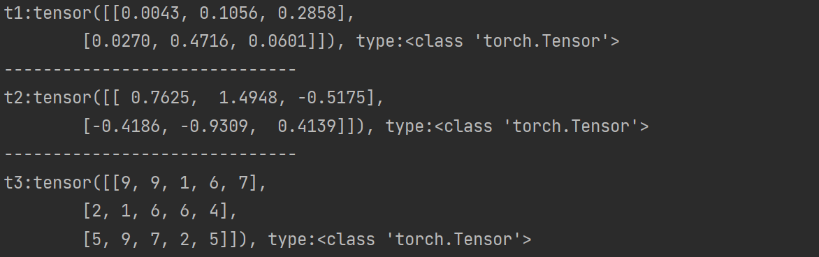
（2）.创建随机张量，设置随机种子initial_seed()、torch.manual_seed( value )以及随机张量rand（）、randn（）和randint（）

{1}.initial_seed()以系统时间戳生成随机种子，不需要传参，一般不用torch.manual_seed( value )需要传参，只要参数一样，那么结果就一样，可重复实验。当设置随机种子后，之后的代码均会被随机种子固定。

#torch.initial_seed()        #默认采用当前系统的时间戳作为随机种子
torch.manual_seed(3)         #设置随机种子

{2}.rand（）为均匀分布，即产生的每个数据都是独立的，数据之间不会影响。size为数据形状（数量）

t1 = torch.rand(size=(2, 3))
print(f't1:{t1}, type:{type(t1)}')

{3}.randn（）为正态分布，均值为0，方差为1。size为数据形状（数量）

t2 = torch.randn(size=(2, 3))
print(f't2:{t2}, type:{type(t2)}')

{4}.randint（）为整数的均匀分布张量，需要传入下限，上限，以及size

t3 = torch.randint(low=1, high=10, size=(3, 5))
print(f't3:{t3}, type:{type(t3)}')

{5}.完整代码

"""
案例：
    演示Pytorch中 如何创建随机和线性 张量

涉及到的函数：
    torch.arange() 和  torch.linspace() 创建线性张量
    torch.random.initial_seed() 和 torch.random.manual_seed()
    torch.rand/randn() 创建随即浮点类型张量
    torch.randint(low, high, size=()) 创建随机整数类型张量

要掌握的函数：arange() linspace()  random.manual_seed() randint(low, high, size=())


"""

# 导包
import torch

#1.创建线性 张量
def dm01():
    #场景1：创建指定范围的线性张量
    # 参1：开始     参2：结束     参3：步长
    t1 = torch.arange(0, 10, 2)
    print(f't1:{t1}, type:{type(t1)}')
    print('_' * 30)
    #场景2：创建指定范围的线性张量  -》等差数列
    #参1：起始     参2：结束     参3：元素个数
    t2 = torch.linspace(1, 10, 4)
    print(f't2:{t2}, type:{type(t2)}')

#2.创建 随机张量
def dm02():
    #step1：设置随机种子
    #torch.initial_seed()        #默认采用当前系统的时间戳作为随机种子
    torch.manual_seed(3)         #设置随机种子

    #step2：设置随机张量
    #场景1：均匀分布的（0， 1）随机张量
    t1 = torch.rand(size=(2, 3))
    print(f't1:{t1}, type:{type(t1)}')
    print('-' * 30)

    #场景2：符合正态分布的随机张量
    t2 = torch.randn(size=(2, 3))
    print(f't2:{t2}, type:{type(t2)}')
    print('-' * 30)

    #场景3：创建随机整数张量
    t3 = torch.randint(low=1, high=10, size=(3, 5))
    print(f't3:{t3}, type:{type(t3)}')


if __name__ =="__main__":
    #dm01()
    dm02()

结果如下图

3.创建全0、1和指定数值的张量

（1）ones 和 ones_like 函数创建全1张量（zeros同理）

ones创建指定形状的张量

t1 = torch.ones(2, 3)  #创建2行3列全1张量
print(f't1:{t1}, type:{type(t1)}')

用ones_like 创建同样形状的张量

#t2：2行3列
t2 = torch.tensor([[1, 2], [3, 4], [5, 6]])
print(f't2:{t2}, type:{type(t2)}')
print('_' * 30)

#t3 ->基于t2的形状，创建全1张量
t3 = torch.ones_like(t2)
print(f't3:{t3}, type:{type(t3)}')
print('_' * 30)

（2）full 和 full_like 创建指定值的张量

t1 = torch.full(size=(2, 3), fill_value=255)  #创建2行3列全255张量
print(f't1:{t1}, type:{type(t1)}')
print('_' * 30)

#t2：2行3列
t2 = torch.tensor([[1, 2], [3, 4], [5, 6]])
print(f't2:{t2}, type:{type(t2)}')
print('_' * 30)

#t3 ->基于t2的形状，创建全255张量
t3 = torch.full_like(t2, 255)
print(f't3:{t3}, type:{type(t3)}')
print('_' * 30)

（3）完整代码

"""
案例：
    演示全0 全1 指定值的张量

涉及到的函数如下：
    torch.ones 和 torch.ones_like    创建全1张量
    torch.zeros 和 torch.zeros_like  创建全0张量
    torch.full  和 torch.full_like   创建全为指定值张量

需要掌握的方式：
    zeros（），full（）
"""

import torch

#场景1：torch.ones 和 torch.ones_like    创建全1张量
t1 = torch.ones(2, 3)  #创建2行3列全1张量
print(f't1:{t1}, type:{type(t1)}')
print('_' * 30)

#t2：2行3列
t2 = torch.tensor([[1, 2], [3, 4], [5, 6]])
print(f't2:{t2}, type:{type(t2)}')
print('_' * 30)

#t3 ->基于t2的形状，创建全1张量
t3 = torch.ones_like(t2)
print(f't3:{t3}, type:{type(t3)}')
print('_' * 30)


#场景2：torch.zeros 和 torch.zeros_like  创建全0张量
t1 = torch.zeros(2, 3)  #创建2行3列全0张量
print(f't1:{t1}, type:{type(t1)}')
print('_' * 30)

#t2：2行3列
t2 = torch.tensor([[1, 2], [3, 4], [5, 6]])
print(f't2:{t2}, type:{type(t2)}')
print('_' * 30)

#t3 ->基于t2的形状，创建全0张量
t3 = torch.zeros_like(t2)
print(f't3:{t3}, type:{type(t3)}')
print('_' * 30)



#场景3：torch.full  和 torch.full_like   创建全为指定值张量

t1 = torch.full(size=(2, 3), fill_value=255)  #创建2行3列全255张量
print(f't1:{t1}, type:{type(t1)}')
print('_' * 30)

#t2：2行3列
t2 = torch.tensor([[1, 2], [3, 4], [5, 6]])
print(f't2:{t2}, type:{type(t2)}')
print('_' * 30)

#t3 ->基于t2的形状，创建全255张量
t3 = torch.full_like(t2, 255)
print(f't3:{t3}, type:{type(t3)}')
print('_' * 30)

4.张量的类型转化

使用 xx.type(torch.xx)来更改张量的类型

#场景1：直接创建指定类型的张量
t1 = torch.tensor([1, 2, 3, 4, 5], dtype=torch.float)       #默认是float32
print(f't1:{t1}, (元素)类型：{t1.dtype},（张量）类型：{type(t1)}')
print('-' * 30)

#场景2：创建好张量后-》做类型转换
#思路1：type（）函数， 推荐掌握
t2 = t1.type(torch.int16)
print(f't2:{t2}, (元素)类型：{t2.dtype},（张量）类型：{type(t2)}')
print('-' * 30)



#思路2：half（）/double（）/float（）/ short（）/ int（）/ long（）
print(t2.half())  #float16
print(t2.double())
print(t2.float())
print(t2.short())
print(t2.int())
print(t2.long())

5.张量与numpy之间的转化

（1）张量转numpy

xx.numpy（），共享内存

 t1 = torch.tensor([1, 2, 3, 4, 5])
 #2.张量 -》 numpy
 #n1 = t1.numpy()                     #共享内存

xx.numpy().copy()，不共享内存

 n1 = t1.numpy().copy()              #不共享内存

（2）numpy转张量

torch.from_numpy(xx)，共享内存

    #1.创建numpy数组
    n1 = np.array([11, 22, 33])
    print(f'n1:{n1}, type:{type(n1)}')

    #2. 把上述的numpy 转化为张量
    t1 = torch.from_numpy(n1)   #默认是n1的类型 即int型 共享内存
    print(f't1:{t1}, type:{type(t1)}')

torch.tensor(xx) ，不共享内存

t2 = torch.tensor(n1)                   #不共享内存
print(f't2:{t2}, type:{type(t2)}')
n1[0] = 100
print(f'n1:{n1}')
print(f't1:{t1}')
print(f't2:{t2}')

（3）从张量中读取内容

xx.item()可以从存有一个数值的张量中读取到数据

#1.创建张量
    t1 = torch.tensor(100.3)            #可以 并且可以输入 True 或者 Flase，映射为 1 / 0 提取出来
    #t1 = torch.tensor([100])            #可以
    #t1 = torch.tensor([100, 200])       #两个数据，不可以 item提取
    print(f't1:{t1}, type:{type(t1)}')
    #2.从张量中 提取内容
    a = t1.item()
    print(f'value: {a}, type:{type(a)}')

（4）完整代码

"""

案例：
    演示张量 和 numpy 之间如何相互转换， 以及 如何从标量张量中 提取其内容

涉及到的API：
    场景1：张量 -》 numpy np数组对象
        张量对象.numpy()            内存共享
        张量对象.numpy（）.copy()    不共享内存   链式编程写法
    场景2：numpy np数组 -》 张量
        from_numpy()                共享内存
        torch.tensor(np数组)          不共享内存
    场景3：从标量张量中 提取其内容
        标量张量.item()
    掌握
    张量-》numpy： 张量对象.numpy（）
    numpy-》张量： torch.tensor（nd数组）
    从标量张量中 提取其内容： 标量张量.item()

"""

import torch
import numpy as np

#1.张量-》 numpy
def dm01():
    #1.创建张量
    t1 = torch.tensor([1, 2, 3, 4, 5])
    #2.张量 -》 numpy
    #n1 = t1.numpy()                     #共享内存
    n1 = t1.numpy().copy()              #不共享内存
    print(f't1:{t1}, type:{type(t1)}')
    print(f'n1:{n1}, type:{type(n1)}')


    #3.演示上述方式 共享内存
    n1[0] = 100
    print(f'n1:{n1}')
    print(f't1:{t1}')



#2.numpy-》张量
def dm02():
    #1.创建numpy数组
    n1 = np.array([11, 22, 33])
    print(f'n1:{n1}, type:{type(n1)}')

    #2. 把上述的numpy 转化为张量
    t1 = torch.from_numpy(n1)   #默认是n1的类型 即int型 共享内存
    print(f't1:{t1}, type:{type(t1)}')
    #t2 = t1.type(torch.float32)
    #print(f't2:{t2}, type:{type(t2)}')
    #或者链时转换
    #t1 = torch.from_numpy(n1).type(torch.float32)   #转换 + 转类型

    t2 = torch.tensor(n1)                   #不共享内存
    print(f't2:{t2}, type:{type(t2)}')
    n1[0] = 100
    print(f'n1:{n1}')
    print(f't1:{t1}')
    print(f't2:{t2}')


#3.从标量张量(只有一个值的张量，如果是多个值则无法提取数据)中 提取其内容：
def dm03():
    #1.创建张量
    t1 = torch.tensor(100.3)            #可以 并且可以输入 True 或者 Flase，映射为 1 / 0 提取出来
    #t1 = torch.tensor([100])            #可以
    #t1 = torch.tensor([100, 200])       #两个数据，不可以 item提取
    print(f't1:{t1}, type:{type(t1)}')
    #2.从张量中 提取内容
    a = t1.item()
    print(f'value: {a}, type:{type(a)}')

if __name__=='__main__':
    #dm01()
    #dm02()
    dm03()

6.张量的基本运算

对于加减乘除取反，都有符号和API两种方式

符号加法

t1 = torch.tensor([1, 2, 3])

#2.演示 加法
t2 = t1.add(10)     #不被修改数据   如果只和一个值运算， 则会将这个值与所有数都进行运算

API方式 add（）不更改原数据 add_（）更改原数据

#1.创建张量
t1 = torch.tensor([1, 2, 3])

#2.演示 加法
t2 = t1.add(10)     #不被修改数据   如果只和一个值运算， 则会将这个值与所有数都进行运算
# t2 = t1 + 10  #效果同上
t3 = t1.add_(10)    #修改原数据
#t1.add_(10)        #会修改原数据
#t1 += 10           #想过同add_ 会修改原数据
print(f't1:{t1}')
print(f't2:{t2}')
print(f't3:{t3}')

完整代码

"""
案例：
    演示张量的基本运算

涉及到的API：
    add（），sub（），mul（），div（），neg（） -》 加减乘除， 取反
    add_（），sub_（），mul_（），div_（），neg_（） ->与上述功能一样， 但是类似于pandas里 inplace = True ，可以替换原数据

需要记忆  1. + - * /  可以代替上述API
         2.如果是张量和数值运算，则：该数值会和张量中的每个值一次进行 对应的运算

"""

import torch

#1.创建张量
t1 = torch.tensor([1, 2, 3])

#2.演示 加法
t2 = t1.add(10)     #不被修改数据   如果只和一个值运算， 则会将这个值与所有数都进行运算
# t2 = t1 + 10  #效果同上
t3 = t1.add_(10)    #修改原数据
#t1.add_(10)        #会修改原数据
#t1 += 10           #想过同add_ 会修改原数据
print(f't1:{t1}')
print(f't2:{t2}')
print(f't3:{t3}')

8.张量的点乘和矩阵乘法

点乘和矩阵乘法也分符合和API两种写法

"""
案例：
    演示张量的点乘  和 矩阵乘法操作

点乘：
    要求：两个张量的维度保持统一， 对应元素直接做 相应的操作
    API：
        t1 * t2
        t1.mul(t2)              #multiply:乘法

        t1 @ t2
        t1.matmul(t2)
        t1.dot(t2)
"""


import torch

#1.点乘
def dm01():
    #1.定义张量，2行3列
    t1 = torch.tensor([[1, 2, 3], [4, 5, 6]])
    #2.定义张量，2行3列
    t2 = torch.tensor([[1, 2, 3], [4, 5, 6]])
    print(f't1:{t1}')
    print(f't2:{t2}')

    #3.演示张量点乘操作   对应元素相乘
    t3 = t1 * t2
    #t3 = t1.mul(t2)        #效果同上
    #4.打印结果
    print(f't3:{t3}')

#2.矩阵乘法
def dm02():
    #1.定义张量，2行3列
    t1 = torch.tensor([[1, 2, 3], [4, 5, 6]])
    #2.定义张量，2行3列
    t2 = torch.tensor([[1, 2], [3, 4], [5, 6]])
    print(f't1:{t1}')
    print(f't2:{t2}')

    #3.演示 张量  矩阵相乘
    t3 = t1 @ t2
    #t3 = t1.matmul(t2)        #效果同上    matrix multiply() 矩阵乘法
    #t3 = t1.dot(t2)             #报错，dot（）只对一维张量有效

    #4.打印结果
    print(f't3:{t3}')

    #5.演示dot函数
    t4 = torch.tensor([1, 2, 3])
    t5 = torch.tensor([4, 5, 6])
    t6 =t4.dot(t5)
    print(f't6:{t6}')       #1*4 + 2*5 + 3*6 = 32

if __name__ =="__main__":
    #dm01()
    dm02()

9.张量的常用运算函数

（1）sum（）

#1.定义张量，记录初值
t1 = torch.tensor([
    [1, 2, 3],
    [4, 5, 6]
], dtype=torch.float)

print(f't1:{t1}')
print('-' * 30)
#2.演示 由dim参数的 函数
print(t1.sum(dim=0))    #按列求和
print(t1.sum(dim=1))    #按行求和
print(t1.sum())         #不传参-》默认整体求和 全加起来

（2）max（）

print(t1.max(dim=0))    #按列求最大值
print(t1.max(dim=1))    #按行求最大值
print(t1.max())         #不传参-》默认整体最大

（3）min（）

print(t1.min(dim=0))    #按列求平均值
print(t1.min(dim=1))    #按行求平均值
print(t1.min())         #不传参-》默认整体求平均值

（4）mean（）

print(t1.mean(dim=0))    #按列求平均值
print(t1.mean(dim=1))    #按行求平均值
print(t1.mean())         #不传参-》默认整体求平均值

（5）pow（）幂函数

print(t1.pow(2))    #每个数的平方
print(t1.pow(3))    #每个数的立方
print(t1 ** 3)         #不传参-》同上
print('-' * 30)

（6）sqrt（）开平方

print(t1.sqrt())
print('-' * 30)

（7）exp（） e的X次幂函数

#exp() e的n次幂， n就是矩阵中每个原色，这里是 e**1， e**2 .。。。 e**6
print(t1.exp())
print('-' * 30)

（8）log（）

#log() log2() log10()
print(t1.log())
print(t1.log2())
print(t1.log10())

（9）完整代码

"""
案例：
    演示张量常用的运算函数
涉及到的API（函数）如下：
    sum， max ， min， mean  -》都有dim参数，0表示列， 1表示行

    pow， sqrt， exp ，log， log2， log10 -》没有dim参数

掌握：
    sum， max， ，min， mean， pow（可以同 a** 5 来代替）

"""

import torch

#1.定义张量，记录初值
t1 = torch.tensor([
    [1, 2, 3],
    [4, 5, 6]
], dtype=torch.float)

print(f't1:{t1}')
print('-' * 30)
#2.演示 由dim参数的 函数
print(t1.sum(dim=0))    #按列求和
print(t1.sum(dim=1))    #按行求和
print(t1.sum())         #不传参-》默认整体求和 全加起来

print('-' * 30)
#演示max
print(t1.max(dim=0))    #按列求最大值
print(t1.max(dim=1))    #按行求最大值
print(t1.max())         #不传参-》默认整体最大

print('-' * 30)
#演示mean 计算平均值
print(t1.mean(dim=0))    #按列求平均值
print(t1.mean(dim=1))    #按行求平均值
print(t1.mean())         #不传参-》默认整体求平均值

print('-' * 30)

#演示 pow 求幂
print(t1.pow(2))    #每个数的平方
print(t1.pow(3))    #每个数的立方
print(t1 ** 3)         #不传参-》同上
print('-' * 30)

#sqrt（） 开平方根
print(t1.sqrt())
print('-' * 30)
#exp() e的n次幂， n就是矩阵中每个原色，这里是 e**1， e**2 .。。。 e**6
print(t1.exp())
print('-' * 30)
#log() log2() log10()
print(t1.log())
print(t1.log2())
print(t1.log10())

10.张量的索引操作

（1）xx[行，列 ] 进行索引

#1.创建随机种子
torch.manual_seed(24)

#2.创建随机张量
t1 = torch.randint(1, 10, (5, 5))
print(f't1: {t1}')
print('-' * 30)

#3.演示张量的索引操作
#场景3：简单行列索引，格式：张量对象[行， 列]      广义上的行列，其中这里的行列还可以单独进行条件选取，具体见场景4
#3.1获取第2行数据
print(t1[1])
print(t1[1, :])  #效果同上
#3.2获取所有行的第3列
print(t1[:, 2])
print('-' * 30)

#场景2：列表索引，前面代表行，后面代表列
#2.1返回（0，1） （1，2）两个位置的数据
print(t1[[0, 1], [1, 2]])
#2.2返回（1，2） （3，4）两个位置
print(t1[[1, 3], [2, 4]])
#2.3获取第0，1行的  1，2列共4个元素
print(t1[[[0], [1]], [1, 2]])

（2）用：可以范围索引：：后可以跟步长

#场景3：范围索引
#3.1前三行，前2列
print(t1[:3, :2])
#3.2:第2行到最后一行， 前2列的数据
print(t1[1: , :2])
#3.3所有奇数行，偶数列,::后＋步长
print(t1[1::2, ::2])
print('-' * 30)

（3）更复杂的条件索引

#场景4：布尔索引    依旧是t1[行， 列]  这里的行和列可以继续增加选取条件
#print(t1[torch.tensor([True, False, False, True, True]), :])    #要第1 4 5 行 所有列
#4.1：第3列 大于5的行数据
print(t1[t1[:, 2] > 5, :])     #t1这个整体中，t1里所有行第3列里 ＞ 5  的所有行
#4.2： 第2行，大于5的 列数据
print(t1[:, t1[1, :] > 5])
print(t1[:, t1[1] > 5])     #效果同上

#在第2行的基础上，找该行所有列中大于5的元素
print(t1[1, t1[1, :] > 5])
print('-' * 30)

（4）多维索引

#场景5：多维索引
#创建3维张量 即：2个 3行4列的矩阵
t2 = torch.randint(1, 10, (2, 3, 4))
print(f't2: {t2}')
#5.1获取0轴上的第1个数据
print(t2[0, :, :])
#5.1获取1轴上的第1个数据
print(t2[:, 0, :])
#5.1获取2轴上的第1个数据
print(t2[:, :, 0])

（5）完整代码

"""
分类：
    简单行列索引
    列表索引
    范围索引
    布尔索引
    多维索引

掌握：
    简单行列索引，范围索引，多维索引

"""

import torch

#1.创建随机种子
torch.manual_seed(24)

#2.创建随机张量
t1 = torch.randint(1, 10, (5, 5))
print(f't1: {t1}')
print('-' * 30)

#3.演示张量的索引操作
#场景3：简单行列索引，格式：张量对象[行， 列]      广义上的行列，其中这里的行列还可以单独进行条件选取，具体见场景4
#3.1获取第2行数据
print(t1[1])
print(t1[1, :])  #效果同上
#3.2获取所有行的第3列
print(t1[:, 2])
print('-' * 30)

#场景2：列表索引，前面代表行，后面代表列
#2.1返回（0，1） （1，2）两个位置的数据
print(t1[[0, 1], [1, 2]])
#2.2返回（1，2） （3，4）两个位置
print(t1[[1, 3], [2, 4]])
#2.3获取第0，1行的  1，2列共4个元素
print(t1[[[0], [1]], [1, 2]])



#场景3：范围索引
#3.1前三行，前2列
print(t1[:3, :2])
#3.2:第2行到最后一行， 前2列的数据
print(t1[1: , :2])
#3.3所有奇数行，偶数列,::后＋步长
print(t1[1::2, ::2])
print('-' * 30)

"""
6 9 9 2 8
7 8 5 8 4
7 4 3 9 3
6 1 4 2 8
1 2 5 7 4

"""

#场景4：布尔索引    依旧是t1[行， 列]  这里的行和列可以继续增加选取条件
#print(t1[torch.tensor([True, False, False, True, True]), :])    #要第1 4 5 行 所有列
#4.1：第3列 大于5的行数据
print(t1[t1[:, 2] > 5, :])     #t1这个整体中，t1里所有行第3列里 ＞ 5  的所有行
#4.2： 第2行，大于5的 列数据
print(t1[:, t1[1, :] > 5])
print(t1[:, t1[1] > 5])     #效果同上

#在第2行的基础上，找该行所有列中大于5的元素
print(t1[1, t1[1, :] > 5])
print('-' * 30)


#场景5：多维索引
#创建3维张量 即：2个 3行4列的矩阵
t2 = torch.randint(1, 10, (2, 3, 4))
print(f't2: {t2}')
#5.1获取0轴上的第1个数据
print(t2[0, :, :])
#5.1获取1轴上的第1个数据
print(t2[:, 0, :])
#5.1获取2轴上的第1个数据
print(t2[:, :, 0])

11.张量的形状

（1）reshape（）

#1.定义2行3列的张量
t1 = torch.randint(1, 10, (2, 3))
print(f't1:{t1}, shape:{t1.shape}, row:{t1.shape[0]}, columns:{t1.shape[1]}, {t1.shape[-1]}') #shape[-1] 代表需要最后一个
#2.通过reshape（）函数， 把t1 -》 3行2列， 1行6列， 6行1列
# t2 = t1.reshape(3, 2)
# t2 = t1.reshape(1, 6)
t2 = t1.reshape(6, 1)
print(f't2:{t2}, shape:{t2.shape}, row:{t2.shape[0]}, columns:{t2.shape[1]}, {t2.shape[-1]}')
#3.尝试通过reshape（）函数，把t1-》2行5列的结果
# t3 = t1.reshape(2, 5)    #报错  转直接 2*3 =6  转之后 2*5 = 10，不一致
# print(t3)

（2）unsqueeze（）和 squeeze（）

unsqueeze（）增加一个向量

#1.定义2行3列的张量
t1 = torch.randint(1, 10, (2, 3))
print(f't1:{t1}, shape:{t1.shape}, row:{t1.shape[0]}, columns:{t1.shape[1]}, {t1.shape[-1]}')
#2.在 0 维上，添加一个维度
t2 = t1.unsqueeze(0)
print(f't2:{t2}, shape:{t2.shape}')
#3.在1维上，添加一个维度
t3 = t1.unsqueeze(1)
print(f't3:{t3}, shape:{t3.shape}')
#4.在2维上，添加一个维度
t4 = t1.unsqueeze(2)
print(f't4:{t4}, shape:{t4.shape}')
# 5.在3维上，添加一个维度
# t5 = t1.unsqueeze(3)        #报错
# print(f't5:{t5}, shape:{t5.shape}')

squeeze（）删除所有1维向量

#6.删除所有为1的维度
t6 = torch.randint(1, 10, (2, 1, 3, 1, 1))
print(f't6:{t6}, shape:{t6.shape}, row:{t6.shape[0]}, columns:{t6.shape[1]}, {t6.shape[-1]}')
t7 = t6.squeeze()
print(f't7:{t7}, shape:{t7.shape}, row:{t7.shape[0]}, columns:{t7.shape[1]}, {t7.shape[-1]}')

（3）transpose（）和 permute（）交换维度且交换后数据都不连续

transpose（）交换两个维度

#1.定义张量
t1 = torch.randint(1, 10, (2, 3, 4))
print(f't1:{t1}, shape:{t1.shape}')
print('-' * 30)
#2.改变维度（2，3，4） -》 （3，2，4）
t2 = t1.transpose(0, 1)
print(f't1:{t1}, shape:{t1.shape}')
print(f't2:{t2}, shape:{t2.shape}')

permute（）交换三个维度数据

#3.改变维度从（2，3，4） -》 （4，2，3）
t3 = t1.permute(2, 0, 1)
print(f't3:{t3}, shape:{t3.shape}')

（4）view（）、contiguous（） is_contiguous（）

view（）交换两个维度并且交换后数据依旧连续

#3.通过view， 修改上述张量的形状
t2 = t1.view(3, 2)
print(f't2:{t2}, shape:{t2.shape}')
print(t2.is_contiguous())

contiguous（）可以使得之前使用transpose和permute不连续的数据连续

#6. 可以通过 contiguous（）函数， 把t3张量 -》 连续张量 -》然后就能通过view修改形状了
t5 = t3.contiguous().view(2, 3)
print(f't5:{t5}, shape:{t5.shape}')

is_contiguous（）可以查看当前数据是否连续

print(t3.is_contiguous())

（5）完整代码

"""
涉及到的API：
    reshape()       在不改变张量内容的前提下，改变形状
    unsqueeze       在指定的轴上增加（1） 个维度，等价于：升维
    squeeze         删除所有为1的维度，等价于：降维
    transpose       一次只能交换两个维度
    permute         一次可以交换多个维度
    view            只能修改连续的张量的形状， 连续张量 = 内存中存储顺序 和 在张量中显示的顺序相同
    contiguous      把不连续的张量 -》 连续的张量 ， 即：基于张量中显示的顺序，修改内存中的存储顺序
    is_contiguous   判断张量是否是连续的

需要掌握：
    reshape、unsqueeze、permute、view

"""


import torch
#1.演示 reshape()函数

torch.manual_seed(24)
def dm01():             #
    #1.定义2行3列的张量
    t1 = torch.randint(1, 10, (2, 3))
    print(f't1:{t1}, shape:{t1.shape}, row:{t1.shape[0]}, columns:{t1.shape[1]}, {t1.shape[-1]}') #shape[-1] 代表需要最后一个维度
    #2.通过reshape（）函数， 把t1 -》 3行2列， 1行6列， 6行1列
    # t2 = t1.reshape(3, 2)
    # t2 = t1.reshape(1, 6)
    t2 = t1.reshape(6, 1)
    print(f't2:{t2}, shape:{t2.shape}, row:{t2.shape[0]}, columns:{t2.shape[1]}, {t2.shape[-1]}')


    #3.尝试通过reshape（）函数，把t1-》2行5列的结果
    # t3 = t1.reshape(2, 5)    #报错  转直接 2*3 =6  转之后 2*5 = 10，不一致
    # print(t3)
#2.演示 unsqueeze（）函数 和  squeeze
def dm02():
    #1.定义2行3列的张量
    t1 = torch.randint(1, 10, (2, 3))
    print(f't1:{t1}, shape:{t1.shape}, row:{t1.shape[0]}, columns:{t1.shape[1]}, {t1.shape[-1]}')

    #2.在 0 维上，添加一个维度
    t2 = t1.unsqueeze(0)
    print(f't2:{t2}, shape:{t2.shape}')
    #3.在1维上，添加一个维度
    t3 = t1.unsqueeze(1)
    print(f't3:{t3}, shape:{t3.shape}')
    #4.在2维上，添加一个维度
    t4 = t1.unsqueeze(2)
    print(f't4:{t4}, shape:{t4.shape}')

    # 5.在3维上，添加一个维度
    # t5 = t1.unsqueeze(3)        #报错
    # print(f't5:{t5}, shape:{t5.shape}')

    #6.删除所有为1的维度
    t6 = torch.randint(1, 10, (2, 1, 3, 1, 1))
    print(f't6:{t6}, shape:{t6.shape}, row:{t6.shape[0]}, columns:{t6.shape[1]}, {t6.shape[-1]}')
    t7 = t6.squeeze()
    print(f't7:{t7}, shape:{t7.shape}, row:{t7.shape[0]}, columns:{t7.shape[1]}, {t7.shape[-1]}')



#3.演示 transpose（）函数permute（）
def dm03():
    #1.定义张量
    t1 = torch.randint(1, 10, (2, 3, 4))
    print(f't1:{t1}, shape:{t1.shape}')
    print('-' * 30)
    #2.改变维度（2，3，4） -》 （3，2，4）
    t2 = t1.transpose(0, 1)
    print(f't1:{t1}, shape:{t1.shape}')
    print(f't2:{t2}, shape:{t2.shape}')

    #3.改变维度从（2，3，4） -》 （4，2，3）
    t3 = t1.permute(2, 0, 1)
    print(f't3:{t3}, shape:{t3.shape}')

#4.演示 reshape()函数view（） contiguous（） is_contiguous（）
def dm04():
    """
    view 无法改变不连续的张量的形状， 可以通过 is_contiguous()判断张量是否连续，
    也可以通过 contiguous 把不连续的张量 -》 连续张量

    """


    #1.定义张量
    t1 = torch.randint(1, 10, (2, 3))
    print(f't1:{t1}, shape:{t1.shape}')
    #判断内存中存储顺序 和 在张量中显示的顺序相同
    print(t1.is_contiguous())

    #3.通过view， 修改上述张量的形状
    t2 = t1.view(3, 2)
    print(f't2:{t2}, shape:{t2.shape}')
    print(t2.is_contiguous())

    #4.通过transpose交换维度 -》交换之后，不连续了
    t3 = t1.transpose(0, 1)
    print(f't3:{t3}, shape:{t3.shape}')
    print(t3.is_contiguous())
    #尝试把 t3张量 从（3， 2）通过view（）转成 （2， 3）
    # t4 = t3.view(2, 3)                  #t3不连续 所以无法改变形状
    # print(f't4:{t4}, shape:{t4.shape}')

    #6. 可以通过 contiguous（）函数， 把t3张量 -》 连续张量 -》然后就能通过view修改形状了
    t5 = t3.contiguous().view(2, 3)
    print(f't5:{t5}, shape:{t5.shape}')

if __name__ == '__main__':
    #dm01()
    #dm02()
    #dm03()
    dm04()

11.张量的拼接

cat（）和stack（）

cat（）要求拼接的两个张量形状一致

#1. 创建两个张量
t1 = torch.randint(1, 10, (2, 3))
print(f't1:{t1}, shape:{t1.shape}')
t2 = torch.randint(1, 10, (2, 3))
print(f't2:{t2}, shape:{t2.shape}')
#2.演示张量拼接
#思路1：cat拼接张量
t3 = torch.cat([t1, t2], dim=0)     #(2,3) + (2,3) = (4,3)  dim=0表示 拼接0维
print(f't3:{t3}, shape:{t3.shape}')
print('-' * 30 )

stack（）要求拼接前两个张量形状一致，合并后也一致，但是会在指定合并轴上多一个维度

#思路2：stack（）拼接张量， 可以是新维度，但是无论新旧维度，所有唯独都必须保持一致
# 1. 创建两个张量
t1 = torch.randint(1, 10, (2, 3))
print(f't1:{t1}, shape:{t1.shape}')
t2 = torch.randint(1, 10, (2, 3))
print(f't2:{t2}, shape:{t2.shape}')
t7 = torch.stack([t1, t2], dim=0)   #(2,3) + (2,3) = (2, 2, 3)
print(f't7:{t7}, shape:{t7.shape}')
t8 = torch.stack([t1, t2], dim=1)  # (2,3) + (2,3) = (2, 2, 3)
print(f't8:{t8}, shape:{t8.shape}')
t9 = torch.stack([t1, t2], dim=2)  # (2,3) + (2,3) = (2, 2, 3)
print(f't9:{t9}, shape:{t9.shape}')

完整代码

"""
案例：
    演示张量的拼接操作

涉及到的API：
    cat（）       不改变维度数，拼接张量，除了拼接的哪个维度外，其他维度数必须保持一致
    stack（）     会改变维度数，拼接张量，所有维度都必须保持一致

"""

import torch
torch.manual_seed(24)

def dm01():
    #1. 创建两个张量
    t1 = torch.randint(1, 10, (2, 3))
    print(f't1:{t1}, shape:{t1.shape}')
    t2 = torch.randint(1, 10, (2, 3))
    print(f't2:{t2}, shape:{t2.shape}')

    #2.演示张量拼接
    #思路1：cat拼接张量
    t3 = torch.cat([t1, t2], dim=0)     #(2,3) + (2,3) = (4,3)  dim=0表示 拼接0维
    print(f't3:{t3}, shape:{t3.shape}')

    print('-' * 30 )

def dm02():
    #思路2：stack（）拼接张量， 可以是新维度，但是无论新旧维度，所有唯独都必须保持一致
    # 1. 创建两个张量
    t1 = torch.randint(1, 10, (2, 3))
    print(f't1:{t1}, shape:{t1.shape}')
    t2 = torch.randint(1, 10, (2, 3))
    print(f't2:{t2}, shape:{t2.shape}')

    t7 = torch.stack([t1, t2], dim=0)   #(2,3) + (2,3) = (2, 2, 3)
    print(f't7:{t7}, shape:{t7.shape}')

    t8 = torch.stack([t1, t2], dim=1)  # (2,3) + (2,3) = (2, 2, 3)
    print(f't8:{t8}, shape:{t8.shape}')

    t9 = torch.stack([t1, t2], dim=2)  # (2,3) + (2,3) = (2, 2, 3)
    print(f't9:{t9}, shape:{t9.shape}')


if __name__ =='__main__':
    #dm01()
    dm02()

12.detach（）将自动微分后的张量转numpy

detcah（）复制的张量共享内存，复制后张量自动微分的属性由T改为F

"""
案例：
    演示detach（）函数的功能，解决 自动微分的弊端


问题：
    一个张量 一旦设置了 自动微分， 这个张量就不能直接转成 numpy的ndarray对象了，需要通过detach（）函数解决

"""

import torch
import numpy as np

#1.定义张量
t1 = torch.tensor([10, 20], requires_grad=True, dtype=torch.float)  #这里设置了自动微分
print(f't1:{t1}, type:{type(t1)}')

#2.尝试把上述的张量 -》 numpy对象
# n1 = t1.numpy()                         #如果数据设置了自动微分， 则无法再直接转了
# print(f'n1:{n1}, type:{type(n1)}')

#3.解决方法：通过detach（）函数，拷贝一份张量，然后转换
t2 = t1.detach()
print(f't2:{t2}, type:{type(t2)}')

#4.测试 上述 t1 和 t2是否共享同一块空间   ->共享空间
t1.data[0] = 100
print(f't1:{t1}, type:{type(t1)}')
print(f't2:{t2}, type:{type(t2)}')
print('-' * 30)

print(f't1:{t1.requires_grad}')
print(f't2:{t2.requires_grad}')

#6.把t2转 numpy对象
n1 = t2.numpy()
print(f'n1:{n1}, type:{type(n1)}')

#最终版本
n2 = t1.detach().numpy( )

三.PyTorch实现线性回归案例

1.数据准备

#1.创建线性回归样本数据
def create_dataset():
    x, y, coef = make_regression(
        n_samples=100,          #样本数
        n_features=1,           #特征数
        noise=10,               #噪声
        coef=True,              #是否返回系数，默认位False
        bias=14.5,              #偏置
        random_state=3          #随机种子

    )

    #print(type(x))
    #把上述 数据集 转化为 张量
    x = torch.tensor(x, dtype=torch.float32)
    y = torch.tensor(y, dtype=torch.float32)


    #3.返回结果
    return x, y, coef

2.模型训练以及结果可视化

#2.模型训练
def train(x, y , coef):
    #1.张量Tensor -》 数据集对象TensorDataset
    dataset = TensorDataset(x, y)
    #参1：数据集对象 参2：批次大小  参3：是否打乱数据（训练集打乱，测试集不打乱）
    dataloader = DataLoader(dataset, batch_size=16, shuffle=True)

    #3.创建初始的 线性回归模型
    #参1：输入特征维度   参2：输出特征维度
    model = nn.Linear(1, 1)

    #4.创建损失函数对象
    criterion = nn.MSELoss()
    #5.创建优化器对象
    #参1：模型参数 参2：学习率
    optimizer = optim.SGD(model.parameters(), lr=0.01)

    #6.具体的训练过程
    #6.1定义变量 分别表示：训练轮数， 每轮的（平均）损失值， 训练总损失值， 训练的样本数
    epochs, loss_list, total_loss, total_sample = 100, [], 0.0, 0
    #6.2开始训练
    for epoch in range(epochs):         #epoch的值：1，2，3，。。。，99
            #6.3每轮是分批次训练的。 所以从 数据加载器中 获取 批次数据
            for train_x, train_y in dataloader: #7批（16， 16， 16， 16， 16， 16， 4）
                #6.4 模型预测
                y_pred = model(train_x)
                #6.5计算(每批平均)损失值
                loss = criterion(y_pred, train_y.reshape(-1, 1))        #-1自动计算 能转多少行转多少行
                #6.6计算总损失 和 样本数（批次数）
                total_loss += loss.item()
                total_sample += 1
                #6.7梯度清零 + 反向传播 +梯度更新
                optimizer.zero_grad()   #梯度清零
                loss.backward()         #反向传播，计算梯度
                optimizer.step()        #梯度更新

            #6.8 把本轮的（平均）损失值 ， 添加到列表中
            loss_list.append(total_loss / total_sample)
            print(f'轮数：{epoch + 1}， 平均损失值：{total_loss / total_sample}')
    #7.打印最终的训练结果
    print(f'{epochs}轮的平均损失分别为：{loss_list}')
    print(f'模型参数， 权重：{model.weight} 偏置：{model.bias}')

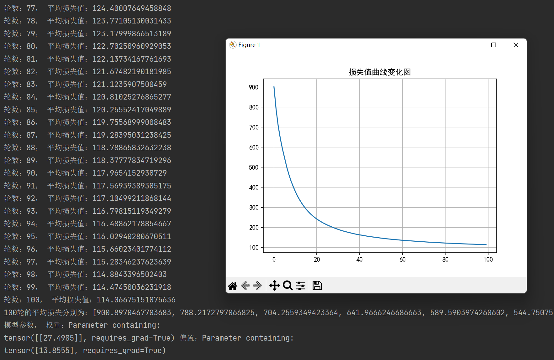
    #8.绘制损失曲线
    #           100lun      每轮的平均损失
    plt.plot(range(epochs), loss_list)
    plt.title('损失值曲线变化图')
    plt.grid()  #绘制网格线
    plt.show()

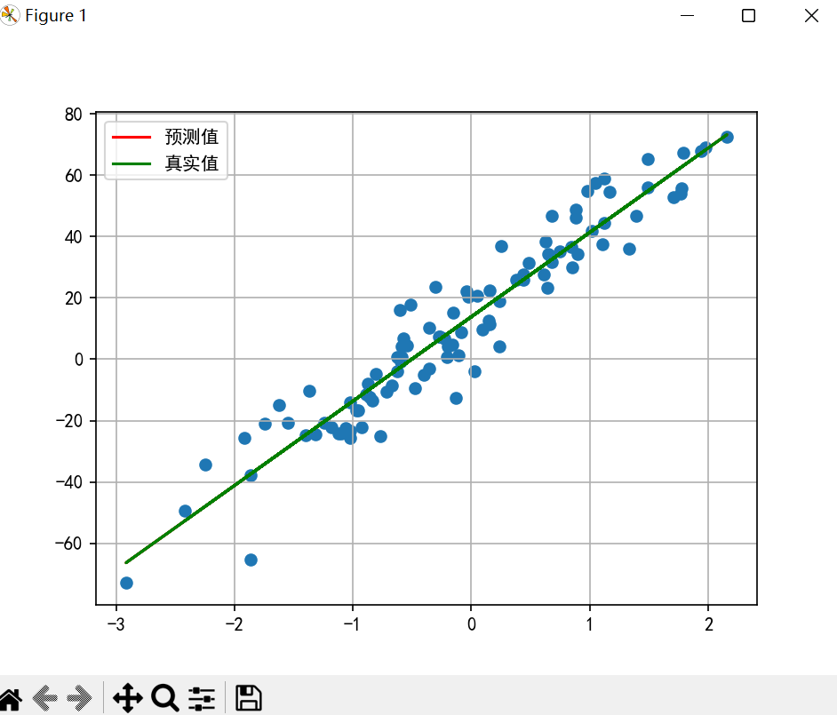
    #9.绘制预测值和真实值的关系
    #9.1绘制样本点分布情况
    plt.scatter(x, y)
    #9.2绘制训练模型的预测值
    #x:100个样本点
    y_pred = torch.tensor(data = [v * model.weight + model.bias for v in x])
    #9.3计算真实值
    y_true = torch.tensor(data = [v * coef + 14.5 for v in x])
    #9.4绘制预测值 和 真实值 的折线图
    plt.plot(x, y_pred, color='red', label='预测值')
    plt.plot(x, y_pred, color='green', label='真实值')
    #9.5图例
    plt.legend()
    plt.grid()  #网格

    plt.show()

3.完整代码

一.pycharm常用快捷键

二.常用函数使用方法

1.张量的基本创建方式

（1）.tensor为最常用的张量创建方法（必须要掌握）

（2）.Tensor的使用方法以及特点

（3）.torch.IntTensor、torch.FloatTensor、torch.DoubleTensor的使用

（4）.完整代码

2.创建线性和随机张量

（1）.创建线性张量，arange（）和linspace（）使用方法

{1}.arange（）创建指定范围的线性张量

{2}.linspace（）创建指定范围的等差线性张量

（2）.创建随机张量，设置随机种子initial_seed()、torch.manual_seed( value )以及随机张量rand（）、randn（）和randint（）

{1}.initial_seed()以系统时间戳生成随机种子，不需要传参，一般不用torch.manual_seed( value )需要传参，只要参数一样，那么结果就一样，可重复实验。当设置随机种子后，之后的代码均会被随机种子固定。

{2}.rand（）为均匀分布，即产生的每个数据都是独立的，数据之间不会影响。size为数据形状（数量）

{3}.randn（）为正态分布，均值为0，方差为1。size为数据形状（数量）

{4}.randint（）为整数的均匀分布张量，需要传入下限，上限，以及size

{5}.完整代码

3.创建全0、1和指定数值的张量

（1）ones 和 ones_like 函数创建全1张量（zeros同理）

（2）full 和 full_like 创建指定值的张量

（3）完整代码

4.张量的类型转化

使用 xx.type(torch.xx)来更改张量的类型

5.张量与numpy之间的转化

（1）张量转numpy

xx.numpy（），共享内存

xx.numpy().copy()，不共享内存

（2）numpy转张量

torch.from_numpy(xx)，共享内存

torch.tensor(xx) ，不共享内存

（3）从张量中读取内容

xx.item()可以从存有一个数值的张量中读取到数据

（4）完整代码

6.张量的基本运算

符号加法

API方式 add（）不更改原数据 add_（）更改原数据

（2）unsqueeze（）和 squeeze（）

（3）transpose（）和 permute（）交换维度且交换后数据都不连续

（4）view（）、contiguous（） is_contiguous（）

12.detach（）将自动微分后的张量转numpy

import torch
from torch.utils.data import TensorDataset                  # 构造数据集对象
from torch.utils.data import DataLoader                     # 数据加载器
from torch import nn                                        # nn模块中有平方损失函数和假设函数
from torch import optim                                     # optim模块中有优化器函数
from sklearn.datasets import make_regression                # 创建线性回归模型数据集
import matplotlib.pyplot as plt                             #可视化

import matplotlib
matplotlib.use('TkAgg')   # 解决后端错误

plt.rcParams['font.sans-serif'] = ['SimHei']                # 用来正常显示中文标签
plt.rcParams['axes.unicode_minus'] = False                  # 用来正常显示负号



#numpy对象 -》 张量Tensor  -》 数据集对象 TensorDataset  -》  数据加载器DataLoader

#1.创建线性回归样本数据
def create_dataset():
    x, y, coef = make_regression(
        n_samples=100,          #样本数
        n_features=1,           #特征数
        noise=10,               #噪声
        coef=True,              #是否返回系数，默认位False
        bias=14.5,              #偏置
        random_state=3          #随机种子

    )

    #print(type(x))
    #把上述 数据集 转化为 张量
    x = torch.tensor(x, dtype=torch.float32)
    y = torch.tensor(y, dtype=torch.float32)


    #3.返回结果
    return x, y, coef

#2.模型训练
def train(x, y , coef):
    #1.张量Tensor -》 数据集对象TensorDataset
    dataset = TensorDataset(x, y)
    #参1：数据集对象 参2：批次大小  参3：是否打乱数据（训练集打乱，测试集不打乱）
    dataloader = DataLoader(dataset, batch_size=16, shuffle=True)

    #3.创建初始的 线性回归模型
    #参1：输入特征维度   参2：输出特征维度
    model = nn.Linear(1, 1)

    #4.创建损失函数对象
    criterion = nn.MSELoss()
    #5.创建优化器对象
    #参1：模型参数 参2：学习率
    optimizer = optim.SGD(model.parameters(), lr=0.01)

    #6.具体的训练过程
    #6.1定义变量 分别表示：训练轮数， 每轮的（平均）损失值， 训练总损失值， 训练的样本数
    epochs, loss_list, total_loss, total_sample = 100, [], 0.0, 0
    #6.2开始训练
    for epoch in range(epochs):         #epoch的值：1，2，3，。。。，99
            #6.3每轮是分批次训练的。 所以从 数据加载器中 获取 批次数据
            for train_x, train_y in dataloader: #7批（16， 16， 16， 16， 16， 16， 4）
                #6.4 模型预测
                y_pred = model(train_x)
                #6.5计算(每批平均)损失值
                loss = criterion(y_pred, train_y.reshape(-1, 1))        #-1自动计算 能转多少行转多少行
                #6.6计算总损失 和 样本数（批次数）
                total_loss += loss.item()
                total_sample += 1
                #6.7梯度清零 + 反向传播 +梯度更新
                optimizer.zero_grad()   #梯度清零
                loss.backward()         #反向传播，计算梯度
                optimizer.step()        #梯度更新

            #6.8 把本轮的（平均）损失值 ， 添加到列表中
            loss_list.append(total_loss / total_sample)
            print(f'轮数：{epoch + 1}， 平均损失值：{total_loss / total_sample}')
    #7.打印最终的训练结果
    print(f'{epochs}轮的平均损失分别为：{loss_list}')
    print(f'模型参数， 权重：{model.weight} 偏置：{model.bias}')

    #8.绘制损失曲线
    #           100lun      每轮的平均损失
    plt.plot(range(epochs), loss_list)
    plt.title('损失值曲线变化图')
    plt.grid()  #绘制网格线
    plt.show()

    #9.绘制预测值和真实值的关系
    #9.1绘制样本点分布情况
    plt.scatter(x, y)
    #9.2绘制训练模型的预测值
    #x:100个样本点
    y_pred = torch.tensor(data = [v * model.weight + model.bias for v in x])
    #9.3计算真实值
    y_true = torch.tensor(data = [v * coef + 14.5 for v in x])
    #9.4绘制预测值 和 真实值 的折线图
    plt.plot(x, y_pred, color='red', label='预测值')
    plt.plot(x, y_pred, color='green', label='真实值')
    #9.5图例
    plt.legend()
    plt.grid()  #网格

    plt.show()




if __name__ == "__main__":
    #3.1创建训练集
    x, y, coef = create_dataset()
    print(f'coef:{coef}')
    print(f'x:{x},y:{y},coef:{coef}')
    #3.2训练模型
    train(x, y, coef)

结果展示