一.Pytorch

1.1新建torch张量，以及查看属性改变形状

新建torch张量：

x= torch.normal(a,b,shape)#生成一个形状为shape，元素均值为a,方差为b的满足正太分布的一个张量

x = torch.arange(20).reshape(4,-1)#元素从0到19

x = torch.zeros(4,4)#还有.ones和.randn

x = torch([[1,2],[2,3]])#也可以自己去写元素

查看张量形状：

print(x.shape,x.numel())

改变张量形状

X = x.reshape(5,-1)

索引和切片

查看张量中元素的总大小：

torch.numel()

1.2张量的计算

基本运算：

一维向量会根据自己的位置自动形成横向量或者列向量参与运算。

x = torch.tensor([1.0, 2, 4, 8])

y = torch.tensor([2, 2, 2, 2])

x + y, x - y, x * y, x / y, x ** y ，x<=>y # **运算符是求幂运算都是对应位置的元素之间的计算torch.exp(x)

将张量按照不同的维度通成一个：

X = torch.arange(12, dtype=torch.float32).reshape((3,4))

Y = torch.tensor([[2.0, 1, 4, 3], [1, 2, 3, 4], [4, 3, 2, 1]])

torch.cat((X, Y), dim=0), torch.cat((X, Y), dim=1)

广播机制：按照维度数为一的维度进行广播

a = torch.arange(3).reshape((3, 1))

b = torch.arange(2).reshape((1, 2))

a, b

1.3节省内存

x[:] = x+y#x的地址不变不分配新内存

x+=y#同上

yield 相当于按下了“暂停键”：

1. 当你在外层用 for X, y in data_iter(...) 调用它时，代码运行到 yield，立刻把这 2 行数据抓出来给你，然后原地冻结，交出 CPU 控制权。

2. 等外层网络把这 2 行数据训练完了，进入下一个循环时，这个函数再原地复活，继续往下走，抓接下来的 2 行。

1.4转化为其他数据类型

#将numpy转化为tensor张量
A = X.numpy()
B = torch.tensor(A)
type(A), type(B)

#将标量张量转化为内置数据类型
a = torch.tensor([3.5])
a, a.item(), float(a), int(a)

1.5线性代数计算

张量乘标量形状不变，元素分别相乘

torch.dot(x,x)#向量点积

torch.mv(s,x)#矩阵和向量相乘

torch.mm(s,v)#矩阵乘法

torch.matmul()#会自动识别两个对象的维度，并调用相应的乘法法则。

A = A.T#矩阵转置

B = A.clone()#分配新内存将A的副本给B

降维：

A.sum()#不论A是几维数据，都按照0、1的唯独顺序倒着相加求和。

A.sum(axis=0)#指定降维的轴

sum_A = A.sum(axis=1, keepdims=True)#指定求合后维度不变

沿某个轴计算A元素的累积总和， 比如axis=0（按行计算），可以调用cumsum函数。 此函数不会沿任何轴降低输入张量的维度。

A.cumsum(axis=0)

范数：一种求和的方式函数

1.向量的范数

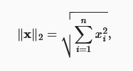
L2级范数：每个元素平方的和再相加

torch.norm(u)

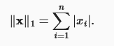
L1级范数：每个元素绝对值的和

torch.abs(u).sum()

2. 矩阵的范数

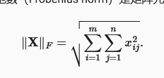
torch.norm(torch.ones((4, 9)))

1.6自动微分

import torch
x = torch.arange(4.0)
x
x.requires_grad_(True)  # 等价于x=torch.arange(4.0,requires_grad=True)
x.grad  # 默认值是None
y = 2 * torch.dot(x, x)
y
y.backward()

分离计算阻断梯度传播

x.grad.zero_()
y = x * x
u = y.detach()
z = u * x

z.sum().backward()
x.grad == u

梯度清零

x.grad.zero_()

以下过程不记录计算图：(即求导的时候不会记录这些计算过程)

with torch.no_grad():

二.Pandas读取数据并转化为tensor（数据预处理）

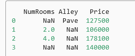
#读取csv数据
data = pd.read_csv(data_file)
print(data)

处理缺失值主要有插值法和删除法：

1.插值法

#用同一列的均值进行替代缺失值、

inputs, outputs = data.iloc[:, 0:2], data.iloc[:, 2]

inputs = inputs.fillna(inputs.mean())

print(inputs)

2.将类别型数据转化为数字表示。对于inputs中的类别值或离散值，我们将“NaN”视为一个类别。 由于“巷子类型”（“Alley”）列只接受两种类型的类别值“Pave”和“NaN”， pandas可以自动将此列转换为两列“Alley_Pave”和“Alley_nan”。 巷子类型为“Pave”的行会将“Alley_Pave”的值设置为1，“Alley_nan”的值设置为0。 缺少巷子类型的行会将“Alley_Pave”和“Alley_nan”分别设置为0和1。

inputs = pd.get_dummies(inputs, dummy_na=True)

print(inputs)

3.将读入的数据转化为tensor类型

import torch

X = torch.tensor(inputs.to_numpy(dtype=float))
y = torch.tensor(outputs.to_numpy(dtype=float))
X, y

三.Matplotlib可视化

plot函数配置：

def use_svg_display():  #@save
    """使用svg格式在Jupyter中显示绘图"""
    backend_inline.set_matplotlib_formats('svg')

def set_figsize(figsize=(3.5, 2.5)):  #@save
    """设置matplotlib的图表大小"""
    use_svg_display()
    d2l.plt.rcParams['figure.figsize'] = figsize

def set_axes(axes, xlabel, ylabel, xlim, ylim, xscale, yscale, legend):
    """设置matplotlib的轴"""
    axes.set_xlabel(xlabel)
    axes.set_ylabel(ylabel)
    axes.set_xscale(xscale)
    axes.set_yscale(yscale)
    axes.set_xlim(xlim)
    axes.set_ylim(ylim)
    if legend:
        axes.legend(legend)
    axes.grid()

#@save
def plot(X, Y=None, xlabel=None, ylabel=None, legend=None, xlim=None,
         ylim=None, xscale='linear', yscale='linear',
         fmts=('-', 'm--', 'g-.', 'r:'), figsize=(3.5, 2.5), axes=None):
    """绘制数据点"""
    if legend is None:
        legend = []

    set_figsize(figsize)
    axes = axes if axes else d2l.plt.gca()

    # 如果X有一个轴，输出True
    def has_one_axis(X):
        return (hasattr(X, "ndim") and X.ndim == 1 or isinstance(X, list)
                and not hasattr(X[0], "__len__"))

    if has_one_axis(X):
        X = [X]
    if Y is None:
        X, Y = [[]] * len(X), X
    elif has_one_axis(Y):
        Y = [Y]
    if len(X) != len(Y):
        X = X * len(Y)
    axes.cla()
    for x, y, fmt in zip(X, Y, fmts):
        if len(x):
            axes.plot(x, y, fmt)
        else:
            axes.plot(y, fmt)
    set_axes(axes, xlabel, ylabel, xlim, ylim, xscale, yscale, legend)

然后调用

x = np.arange(0, 3, 0.1)
plot(x, [f(x), 2 * x - 3], 'x', 'f(x)', legend=['f(x)', 'Tangent line (x=1)'])即可绘制二维图像的切线图

四.Random

#随机打乱数组

x = list(range(n))

random.shuffle(x)